Chapter 12: Random Numbers and Monte Carlo Simulations

Return to all notes

Monte Carlo Simulations

One big part of scientific computation is the subject of Monte Carlo simulations in which random numbers are used to model some situation. We’ll spend the next part of this course covering this subject.

Probability

To fully understand how to use random numbers and how Monte Carlo simulations work, we need some basic probability. When understanding probability there are two types continuous and discrete, which for what we need will come down to using floating point or integers.

###Discrete Probability

We’ll first discuss discrete probability. A discrete probability distribution is a finite set (often will be a subset of integers.) For example, let’s use the set

\[A=\{1,2,3,4,5,6\}\]

and an event, $X$ is subset of these numbers. For example, let $X={1}$, then the probability that this event occurs in the ratio of the number of elements in each set or \(P(X)=\frac{N(X)}{N(A)}\)

In this case, $P(X)=1/6$ and that means that the probability that the number 1 comes up is 1/6. Think about this in the case of rolling a die. This says that the probability that 1 comes up is 1/6.

###Continuous Probability

Another type of probability distribution is called a continuous distribution and in this case we’ll only consider a type of continuous probability distribution called a uniform distribution.

Let’s consider a set $A={x \;

\; 0 \leq x \leq 1}$ or all real numbers between 0 and 1. Events are still subsets of the set $A$, however the probability that events occur is the fraction of the set.

For example, if $X={x \; | \; 1/3 \leq x \leq 1/2}$, then $P(X)$ is the fraction \(P(X) = \frac{\frac{1}{2}-\frac{1}{3}}{1-0}=\frac{1}{6}\)

Pseudo Random Number Generator

The Wikipedia Pseudo-random Number Generator page gives an overview of the subject and a lot of technical details. In short, a truly random number on a computer is very difficult to generate and generally not necessary because a pseudorandom number is sufficient. I also won’t try to explain this in general term since you’d need a significant mathematical background.

A pseudo-random number generator is a function that produces a sequence of numbers that act like random numbers. Let’s examine what this means in terms of the discrete probability with set $A={1,2,3,4,5,6}$.

If a pseudo-random number generator produces a sequence from this set then the sequence should have the following property:

• If the event $X={i}$ for any $i$ between 1 and 6, then $P(X)\approx 1/6$. And by approximately, as the sequence gets larger, the approximation becomes closer to 1/6.

Is this enough? No, the sequence \(\{1,2,3,4,5,6,1,2,3,4,5,6,\ldots\}\)

satisfies the above property, but I don’t think anyone would consider this random. Another property would be:

• If we know the sequence ${a_1,a_2,a_3,\ldots,a_n}$ then we can’t predict the next number $a_{n+1}$.

This is obviously violated in the sequence above.

A little more technical definition of a sequence of pseudo-random numbers Let $(a_1,a_2,a_3, \ldots)$ be a random sequence. Typically we mean the following properties need to hold:

1. any number in the range 1 to 6 is equally likely to occur.
2. Take N random numbers and let $s_n$ be the number of times the number $n$ occurs. The fraction $s_n/N$ should go to 1/6 in the limit as $n\rightarrow \infty$.
3. Knowing the sequence $s_1, s_2, \ldots, s_k$ does not allow us to predict $s_{k+1}$

If instead we use floating point numbers, there are a few different properties. Assume that the floating point number is in the range $0 \lt x \lt 1$. Then the sequence $(a_1,a_2,a_3, \ldots)$ is random if

1. Let $s_{[c,d]}(a_1,a_2,a_3, \ldots)$ be the total of the numbers that satisfy $c \lt a_k \lt d$. Then as the number of random numbers approach infinity $s_{[c,d]}=d-c$

Using Julia to simulate the rolling of a die

First, the main commands that are built-in to Julia are listed in the Julia Manual for Random Numbers. We can generate 100 random numbers between 1 and 6 using

S=rand(1:6,100)

and notice that if you rerun the command, you’ll get a different sequence of random numbers. We can check that this is doing what we expect by checking the probability that we get a 1 (or any other number).

To check the count of the number 1 that appears, try

count(a->a==1,S)

###Exercise

Convert this to a probability. Is it close to what you expect? Try changing the number of random numbers used to larger numbers. Does your answer get closer to what you expect?

Floating Point random numbers

Let’s look a floating point random numbers between 0 and 1. To generate a sequence (array) of such numbers, type

S=rand(100)

and we can check the number of values less than 0.1 with the command:

count(a->a<0.1,S)

and if we want the number of values between 0.4 and 0.7 then type

count(a->0.4<a<0.7,S)

###Exercise

Change the number of random numbers used to much larger set and return the above commands. What are the results? Is this what you expect?

How to do find the fraction of number that are less that 0.25 and greater than 0.75?

The mapslices commands

Below we will encounter another nice function that we can use with arrays. If we have the following array:

A = [1 2 3; 4 5 6; 7 8 9]

and we wish to sum the rows. For any given row, this isn’t difficult. If we want to do all of the rows and return a 1D array (vector), we can use the mapslices function. See the julia documentatation on mapslices.

mapslices(sum,A; dims = [2])

returns the column vector [6,15,24] which are the row sums and

mapslices(sum,A; dims = [1])

returns the row vector [12,15,18] or the column sums.

Exercise

For the matrix above, find the result if you multiply the rows together. Do the same for the columns.

Other Examples

Rolling 2 dice

How do we handle the rolling of two dice? Here’s an array with each row having 2 dice.

S=rand(1:6,100,2)

and then to find the sum of the dice:

dicesum = mapslices(sum,S;dims=[2])

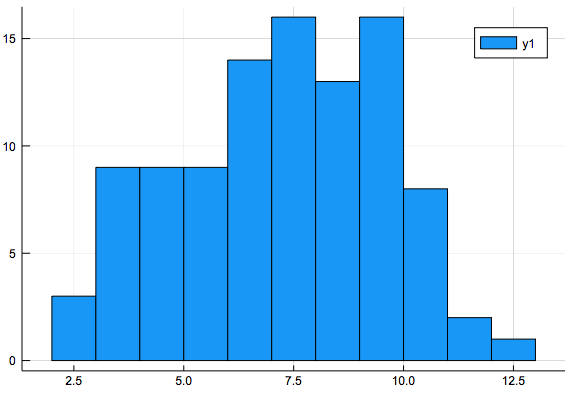
which sums along the rows. This is 100 rolls of 2 dice with the sum recorded. First, to get an idea of the distribution of the dice sums, let’s plot the results using Plots. So first, load it in

using Plots
gr()

or use your favorite backend.

and then to plot the sum

histogram(dicesum,nbins=11)

where nbins is the number of bins and in this case, since it runs from 2 to 12, there’s a total of 11.

generates the following plot:

We could find the number of 2’s 3’s, etc. using the mapslices function as above, however there is a nice way to do this use the StatsBase package. You may need to add the package and then load it with

using StatsBase

and then the counts function ( Read the online documentation) can be used:

counts(dicesum,2:12)

returns a vector of how many of the dice sum fall into each number.

###Exercise

Change the code above to use 1000 dice rolls. Estimate the probability that you

• roll a 7.
• roll a 10 or greater.
• roll an even number.

Plot a the histogram using 1000 dice rolls.

Calculating $\pi$ using pseudo random numbers

• Buffon’s Needle Experiment (18th C.)

• Circle in the Square.

  Consider the square ${ (x,y)\;

  \; 0\leq x\leq 1, 0 \leq y \leq 1}$ and the quarter circle that falls within $x^{2}+y^{2} \leq 1$. The area within the circle is the fraction of the cirle in the square or $\pi/4$.

  We can use this to estimate a value of $\pi$.

  1. Randomly choose points $x$ and $y$ in the range [0,1].
  2. Count all points that fall within the circle.
  3. Find the fraction of the points in the circle.
  4. Since this fraction should be $\pi/4$, multiply by 4 to estimate $\pi$.

  This can be done in julia using

  1. S1=rand(100,2)
  2. S2 = mapslices(x->x[1]^2+x[2]^2,S1; dims=[2])
  3. S3 = count(a->a<1,S2)
  4. fr=S2/100
  5. est=4*fr

  or combine all of these into one command:

    4*count(a->a<1,mapslices(x->x[1]^2+x[2]^2,rand(100,2); dims=[2]))
  

Exercises

• Write a function that take a positive integer $n$, in and performs the approximate-$\pi$ calculation described above using $n$ points. It should return the approximate value of $\pi$.

• Test it will high values of $n$ and time it.

• for $N=10^5$, $N=10^6$ and $N=10^7$ find the relative error of the estimate using your function and using the built-in value pi.