| Previous Chapter | Return to all notes |
Complex Numbers
Recall that the imaginary unit $i$ is defined as the number such that $i^{2}=-1$. In Matlab, we create imaginary number with
im = complex(0,1)
which returns 0.0000+1.000i. The complex function creates a complex number where the first argument is the real part and the second argument is the imagainary part. If we square this with
im^2
and you get $-1$.
Arithmetic with complex numbers
Matlab can handle standard arithmetic operations with complex nubmers. Just to recall if \(z_1=x_1+i y_1 \qquad z_2 = x_2 + i y_2\)
then \(\begin{array}{rl} z_1 + z_2 & = (x_1+x_2) + i(y_1+y_2)\newline z_1 - z_2 & = (x_1-x_2) + i(y_1-y_2) \newline z_1 z_2 & = (x_1+iy_1)(x_2+iy_2) \newline & = (x_1x_2+iy_1x_2+ix_1y_2+i^{2}y_1y_2)\newline & = (x_1x_2-y_1y_2)+i(x_1y_2+x_2y_1) \end{array}\)
Also, if we have $1/z_1$, then we can write this as \(\begin{array}{rl} \dfrac{1}{z_1} & = \dfrac{1}{x_1+iy_1} \end{array}\) mulitply top and bottom by $\overline{z_1}$ \(\begin{array}{rl} \dfrac{1}{z_1} = \dfrac{1}{z_1}\dfrac{\overline{z_1}}{\overline{z_1}} & = \dfrac{1}{x_1+iy_1} \dfrac{x_1-iy_1}{x_1-iy_1} \\ &= \dfrac{x_1-iy_1}{x_1^{2}+y_1^{2}} \end{array}\) and in a similar manner: \(\begin{array}{rl} \dfrac{z_1}{z_2} & = \dfrac{x_1+iy_1}{x_2+iy_2} \\ & = \dfrac{x_1+iy_1}{x_2+iy_2} \dfrac{x_2-iy_2}{x_2-iy_2} \\ & = \dfrac{x_1x_2+y_1y_2+i(y_1x_2-y_2x_1)}{x_2^{2}+y_2^{2}} \end{array}\)
An integer power of a number is found by successive multiplications. For example, \(z^{2} = (x+iy)(x+iy)=x^{2}-y^{2}+2xy i\)
Matlab can do all of these operations naturally. For example, if
z1=complex(3,4)
z2=complex(2,-2)
Then z1+z2 returns ans = 5.0000 + 2.0000i, z1-x2 returns ans = 1.0000 + 6.0000i, z1*z2 returns ans = 14.0000 + 2.0000i and z1/z2 returns
ans = -0.2500 + 1.7500i
z1^2 returns ans = -7.0000 + 24.0000i
The Complex Plane
The complex plane is just like the $xy$-plane in which the horizontal axis is the real axis and the vertical one is the imaginary axis. We can plot any point $x_1+i y_1$ as the point $(x_1,y_1)$ on the standard $xy$-plane.
(add a plot)
The real an imaginary parts of a complex number
If $x$ and $y$ are real numbers and we define $z=x+iy$, then there are functions that return the real and imaginary parts of $z$. Mathematically, we use $\Re(z)$ and $\Im(z)$ to represent these and they are defined as
\[\Re(z)=x \qquad \Im(z)=y\]and note that the imaginary part of a complex number is a real number.
In Matlab, we use the commands real and imag return the real and imaginary parts of a complex number.
z = complex(3,4)
then real(z) returns 3 and imag(z) returns 4.
The Polar Form of a complex number
Another important form of a complex number is called the polar form. If we find $r$, the distance from the origin to the point $(x,y)$ and $\theta$, the counterclockwise angle between the positive $x$ axis and the line segment as shown
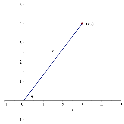
The distance $r$ is defined as $r=\sqrt{x^{2}+y^{2}}$ and $\theta = \tan^{-1} (y/x)$ (and it might need to be shifted depending on the quadrant of the point.)
| In addition, the distance $r$ is often denoted as $ | z | $, where the standard absolute value symbol is used. |
Matlab uses the absolute value function abs for the distance and the angle command for the angle. For example, abs(z) returns 5 and angle(z) returns 0.9273, the angle (in radians).
Complex Conjugate
If $z=x+iy$, then the complex conjugate of $z$, denoted $\overline{z}$ is $x-iy$. In short, it switches the sign of the imaginary term.
In Matlab, the command conj will return the complex conjugate.
conj(z)
returns 3.0000 - 4.0000i
Note that it is common that a complex number is mutiplied by its conjugate, so \(\begin{array}{rl} z \overline{z} & = (x+iy)(x-iy) \\ & = x^{2} +ixy-ixy-i^{2}y^{2} = x^{2}+y^{2}\end{array}\)
| which is $ | z | ^2$, the square of the distance. |
Complex Exponential form
Using the distance and angle of a complex number, we can write a number $z$ as \(z = r e^{i \theta}\) because \(e^{i \theta} = \cos \theta + i \sin \theta\) so, \(\begin{array}{rl} z & = r (\cos \theta + i \sin \theta) \newline & = r \cos \theta + i r \sin \theta \newline & = x + i y \end{array}\)
Multiplication and Powers of Complex Numbers in Polar Form
If we write \(z_1 = r_1 e^{i \theta_1} \qquad z_2 = r_2 e^{i \theta_2}\)
then \(\begin{array}{rl} z_1 z_2 & = r_1 e^{i \theta_1} r_2 e^{i \theta_2} \newline & = r_1 r_2 e^{i(\theta_1+\theta_2)} \end{array}\) or in other words, the product of two complex numbers is found by multiplying the distances and the angle is the sum.
We can find the product of $z_1 = 1+i$ and $z_2 = 2i$ using the above method, or write \(z_1 = \sqrt{2} e^{i\pi/4} \qquad z_2 = 2 e^{i\pi/2}\)
and \(\begin{array}{rl} z_1z_2 & = r_1 r_2 e^{i(\theta_1+\theta_2)} \newline & = 2\sqrt{2} e^{i 3\pi/4} \end{array}\)
The two numbers on the right side of the plot are multiplied. The sum of the angle is $3\pi/4$, which is the angle of the resultant. The distance of the resultant is the product of the two $\sqrt{2}$ and $2$.
The powers of a complex number also have an interesting geometry. If $z=1+i=\sqrt{2}e^{i\pi/4}$, then powers of $z$ can be written as \(z^{n} = (\sqrt{2})^{n} e^{i n \pi/4}\)
This can be interpreted as raising the distance to the $n\text{th}$ power and rotating the angle $n$ times around. For example, the plot about actually shows the number and its 2nd and 3rd power.
If the power is a fraction, we can interpret the same way. For example, the square root of $z$ can be written: \(\sqrt{z} = \sqrt{r e^{i\theta}} = \sqrt{r} e^{i\theta/2}\)
What this means is that to find the square root of a complex number, you take the square root of the distance and then return the number with angle half of the input.
Example
Find the square root of $z=-1+\sqrt{3}i$. Note that $|z|=\sqrt{1^{2}+(-\sqrt{3})^{2}}= \sqrt{4}=2$ and that the angle (argument) is $2\pi/3$. The resultant would have distance $\sqrt{2}$ and the angle would be $\pi/3$ so \(\sqrt{z} = \sqrt{2}e^{i\pi/3}\)
Fundamental Theorem of Algebra
Roots of unity
An interesting function to study in complex numbers is $f(z)=z^{n}-1$ for positive integers $n$. When $n=2$, we get the function $x^{2}-1$ which isn’t that interesting, but not bad. Note that the roots of this are $x=\pm 1$. Let’s look at the solution to $f(z)=z^{3}-1$.
A good way to do this is to recall that we can write $z$ in its polar form or \(z=re^{i\theta}\) and then we want to solve \(z^{3}-1 = r^{3} e^{3i\theta}-1\) Since we can write $1=1e^{0 i}$, then \(r^{3} e^{3i\theta} = e^{0i}\) results in $r^{3}=1$ or $r=1$ and $\theta=0$. This is the number $z_1=1$ and we know that $1^{3}-1=0$. What else?
We can also write $1=e^{2\pi i}$ so \(3i \theta = 2\pi i\) or $\theta=2\pi/3$, so another root of $f$ is \(z_2=e^{2\pi/3 i}\)
and lastly, we can also write $1=e^{4\pi i}$ so another root when $\theta=4\pi/3$ or the number \(z_3=e^{4\pi/3}\)
These points are on the unit circle and equally spaced with $z=1$ a root. This is true in general for functions of the form $f(z)=z^{n}-1$, which will have the roots on the unit circle equally spaced $2\pi/n$ radians apart from each other.
General solution to the roots of unity
The solutions in the complex plane to the equation $f(z)=z^n-1$ are called the roots of unity. We will use the technique above to find the solution.
First, recall that the fundamental theorem of algebra states that there are exactly $n$ complex solutions to a degree $n$ polynomial (including multiplicities), so we expect $n$ solutions to this. \(\begin{aligned} z^n &= 1 \\ & = e^{2k\pi i} \qquad \text{for $k=0,1,2,\ldots,n-1$} \\ z & = e^{(2\pi k)/n i} = \cos \left(\frac{2k\pi}{n}\right) + i \sin \left(\frac{2k\pi}{n}\right) \end{aligned}\) And these values are on the unit circle, one of which is $z=1+0i$ and the others are equally spaced around the circle.
Example
If $n=3$, then the values are \(\begin{aligned} z & = 1+0i, \cos(2\pi/3) + i \sin (2\pi/3), \cos(4 \pi/3) + i \sin (4\pi/3) \\ & = 1+0i, -\frac{1}{2} + i\frac{\sqrt{3}}{2}, -\frac{1}{2} - i\frac{\sqrt{3}}{2} \end{aligned}\)
Newton’s Method in the Complex Plane
In Chapter 13, we met Newton’s method. It works with complex numbers as well. For example, consider the function \(f(x)=x^{2}+4\) which does not have a root in the reals. If we use
newton(x^2+4, 1)
we get the warning: The maximum number of steps have been reached and a result -4.8018.
Newton’s method with Complex numbers
I have updated the Newton’s method function as the following:
function result = newton(f,x0,options)
  arguments
    f function_handle
    x0 (1,1) {mustBeNumeric}
    options.eps (1,1) {mustBePositive} = 1e-6
    options.max_steps (1,1) {mustBePositive} = 10
  end
  syms x
  df(x) = diff(f(x),x);
  x1=x0;
  steps=0;

  dx=double(1); % this will be a step, just initialized to 1 to get the while loop started
  while abs(dx)>options.eps && steps < options.max_steps
    dx=double(f(x1)/df(x1));
    x1 = x1-dx;
    steps = steps + 1;
    if steps == options.max_steps
        warning("The maximum number of steps have been reached.");
    end
  end
  result = x1;
end
and again, it is preferable to save this as a .m file and if it is in a separate directory don’t forget the addpath function.
This updated version of newton’s method allows us to use complex numbers so if we put in a complex number as an input then we will get a complex result.
newton(@(x) x.^2+4,complex(0,1))
we now get 0.0000 + 2.0000i as the result and this makes since because $(2i)^2+4 = -4+4=0$.
Return to Newton’s method
We’re going to apply Newton’s method to find roots of $f(z)=z^{3}-1$.
Exercise
Apply Newton’s method on this function for the following initial points:
- $z=0.1$
- $z=-i$
- $z=i$
- $z=-1$
- $z=0.5 i + 0.5$
Each of these will go to one of the 3 roots. To get a nice representation of this, we are going to do this for many points in the complex plane and color code the results. For example, the first and fourth point can be red, the 2nd and 5th points blue and the 3rd point green.
We now want to do this for many points in the complex plane. There are some nice built-in functions in Matlab to allow us to do this easily. The following:
[X,Y] = meshgrid(-3:0.5:3,3:-0.5:-3);
creates a grid of $x$ and $y$ values. Note to get the grid setup in a way that is consistent with our understanding of the complex plane, the second argument goes from 3 to -3 with steps of -0.5. We can then create a grid of complex values with
complex(X,Y)
which an 13 by 13 array with complex numbers arranged on a grid.
We next want to apply Newton’s method to every number in the Matrix. If we do that, the point in the center will return an error, so we:
Z(7,7) = complex(0.0001,0.0001)
which is close to 0, but not exactly. Then run newton’s method on all of the points in Z using
roots=arrayfun(@(z) newton(@(x) x.^3-1,z),Z)
and you’ll notice that there are warning because we didn’t get close, but changing this to
roots=arrayfun(@(z) newton(@(x) x.^3-1,z,'max_steps',100),Z)
results in no error, but slows down the calculation.
The array roots results in the root that newton’s method has converged to for each starting point. For example, the first row, first column $-3+3i$ converges to $-1$.
A relatively simple way to determine the root each goes to is to find the angle using
arrayfun(@(r) angle(r),roots)
and notice that this is in radians. We can switch to degrees with
arrayfun(@(r) angle(r),roots)*180/pi
however there are repeated values like -180 and 180 and and others that are the same angle. We can shift everything to 0 to 360 with
mod(arrayfun(@(r) angle(r),roots)*180/pi,360)
Finally, we will plot each angle with a different color using:
image(angles,'CDataMapping','scaled')
which generates the plot:
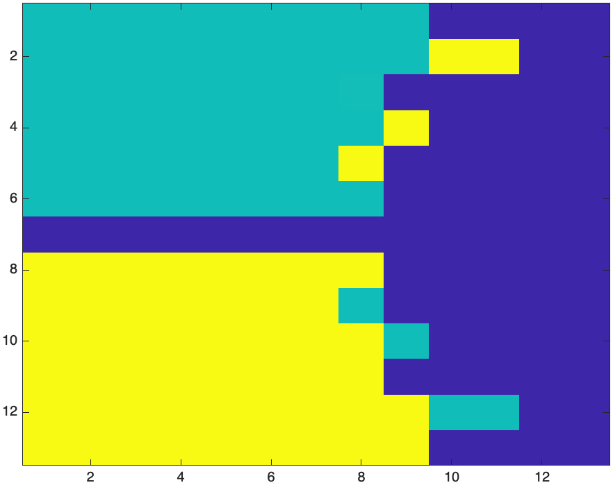
All of the dark blue squares go to the root at $1$. The aquamarine go to the root at $-\sqrt{3}/2 + i/2$ and the yellow go to $-\sqrt{3}/2 - i/2$.
Producing the same plot with a denser grid
[X,Y] = meshgrid(-3:0.01:3,3:-0.01:-3);
Z=complex(X,Y);
Z((size(Z,1)-1)/2,(size(Z,2)-1)/2)=complex(0.0001,0.0001);  % make the center point just off of zero.
for i=1:25  % run newton's method 25 times.  Don't worry about stopping if it converges
    Z = Z-(Z.^3-1)./(3*Z.^2);
end
Z
and we find the angle of each point with
angles = mod(arrayfun(@(r) angle(r),Z)*180/pi,360);
angles(find(angles>359))=0;
and finally plot the angles with
image(angles,'CDataMapping','scaled')
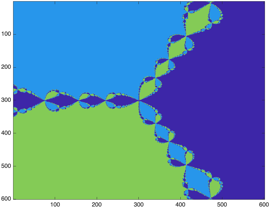
colorbar
The result is
and the following will improve the appearance of the plot:
xticks(0:100:600)
xticklabels(-3:3)
yticks(0:100:600)
yticklabels(3:-1:-3)
axis equal
the result is
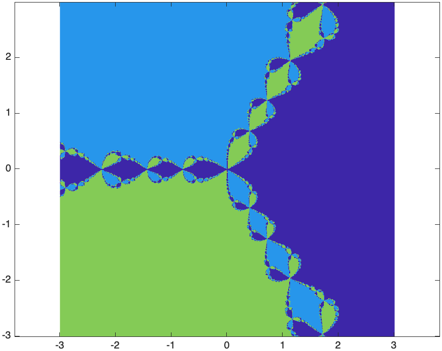
An astute eye will pick up that near the cusps throughout the plot that things look blurry. This is because Newton’s method hasn’t converged yet for these points. If you rerun this with 50 iterations of newton’s method (change the 10 in the for loop above to 50, you’ll get)
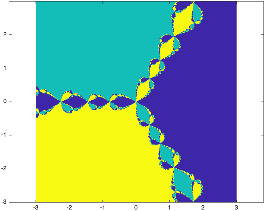
This is an example of a fractal, which is a geometric figure that is self-similar at multiple scales. This means that if you look at the image at various levels, it looks very similar. Related, a fractal generally has infinite detail. Typically, as you zoom in, you will continue to see more an more detail.