Chapter 18: Shortest Paths through a Graph and the Traveling Salesperson Problem
The Traveling Salesperson Problem
A classic example of a minimum problem is that of the traveling salesperson problem or TSP. The problem goes like this: a salesperson needs to visit N cities on her route. There is a known distance between all pairs of the cities. What is the path she should take to minimize the total distance.
Although such a problem may seem a bit archaic (at least the name is). There are many problems that fit into this and in fact, when you use a mapping program to find the shortest route somewhere, at some level, there is a TSP in there somewhere.
Here’s how it goes. The following in a complete graph in that 1) the graph is a set of nodes and edges that connect the nodes. 2) it is complete because any nodes is connected to all other nodes:

Let’s say that the nodes are labelled from A (top) clockwise to E (upper left). And then the distances between the nodes (also called the weights) are given by the following table:
| Node 1 | Node 2 | Distance |
|---|---|---|
| A | B | 26 |
| A | C | 19 |
| A | D | 39 |
| A | E | 23 |
| B | C | 13 |
| B | D | 21 |
| B | E | 42 |
| C | D | 32 |
| C | E | 25 |
| D | E | 17 |
Again, the question is: What path through all of the nodes leads to the smallest total distance. For example, if we choose A->B->C->D->E->A, the the total distance is 26+13+32+17+23=111
Exhaustive Solution (or Brute Force)
In this case, there aren’t that many total paths. With 5 nodes, there are a total 24 different paths and that’s not too difficult to traverse. Let’s look on how to do this in Julia.
First, let’s put the distances into an array:
distances5=
[0 26 19 39 23;
26 0 13 21 42;
19 13 0 32 25;
39 21 32 0 17;
23 42 25 17 0]
where we’ve assumed that the distance of a node to itself is 0 and the matrix is symmetric because the distance from A to B is the same as from B to A.
Next, let’s define a function that finds the total distance given a array of node numbers:
"given the path in the argument nodes, find the total distance travelled."
function total_distance(nodes::Array{Int,1},distances::Array{T,2}) where T<: Real
  local sum=distances[nodes[1],nodes[end]] # add in the distance from first to last
  for i=1:length(nodes)-1
      sum+=distances[nodes[i],nodes[i+1]]
  end
  sum
end
As a test if we pass the totalDistance the array [1 2 3 4 5], we should get the result 111.
total_distance(collect(1:5),distances5)Permutations
This is a bit of a side conversation about permutations. In short, to permute objects means to rearrange their positions. Although permutations has a bigger scope and you can see the Wikipedia page on Permutations for more information, we are going to concentrate here on permuting the entries in a vector. Here are the following permutations of (1,2,3): (1,2,3),(1,3,2),(2,1,3),(2,3,1),(3,1,2),(3,2,1).
There are 6 total here and in general, there are $n!$ permutations of a vector of length n. Julia has some nice built-in functions to create permutations. For example to create the 6 permutations listed above, we first need to load the Combinatorics package:
using Combinatoricsfor i=1:6
println(nthperm(collect(1:3),i))
endwe use the nthperm command which needs a vector and an integer.
A vector of anything can be permuted. Here’s an array of strings.
for i=1:24
    println(nthperm(["horse","zebra","camel","whale"],i))
end
which returns:
["horse", "zebra", "camel", "whale"]
["horse", "zebra", "whale", "camel"]
["horse", "camel", "zebra", "whale"]
["horse", "camel", "whale", "zebra"]
["horse", "whale", "zebra", "camel"]
["horse", "whale", "camel", "zebra"]
["zebra", "horse", "camel", "whale"]
["zebra", "horse", "whale", "camel"]
["zebra", "camel", "horse", "whale"]
["zebra", "camel", "whale", "horse"]
["zebra", "whale", "horse", "camel"]
["zebra", "whale", "camel", "horse"]
["camel", "horse", "zebra", "whale"]
["camel", "horse", "whale", "zebra"]
["camel", "zebra", "horse", "whale"]
["camel", "zebra", "whale", "horse"]
["camel", "whale", "horse", "zebra"]
["camel", "whale", "zebra", "horse"]
["whale", "horse", "zebra", "camel"]
["whale", "horse", "camel", "zebra"]
["whale", "zebra", "horse", "camel"]
["whale", "zebra", "camel", "horse"]
["whale", "camel", "horse", "zebra"]
["whale", "camel", "zebra", "horse"]
Exploring all cases of the TSP
Returning to the Traveling Salesperson Problem (TSP), the example above has 5!=120 permutations or different paths. An exhaustive search of the TSP is simply passing every permutation of the vector [1 2 3 4 5] to the total_distance function. Then you search for the smallest total distance.
If we first find all of the permutations:
perms=map(k->nthperm(collect(1:5),k),collect(1:factorial(5)))then we can find the distance for each:
all_distances=map(p->total_distance(p,1.0*distances5),perms)To find the smallest distance, we use:
findmin(all_distances)which returns (93,7) meaning that the value 93 is the smallest distance and it occurs in the 7th place. To determine the path, apply the nthperm function again:
perms[7]which results the path [1 3 2 4 5] or A->C->B->D->E .
Note: there are other shortest paths, but this is just because you start in different places. For example D->B->E->E->A is also one.
We don’t need to search everything
As we showed above, any solution will have each node in it. We can then always take the first node (A or 1) to be in the first location. This way we can just search the first 4! permutations (this will always have A first).
If we repeat our search in a more compact way using:
dist=map(k->total_distance(nthperm(collect(1:5),k),1.0*distances5),1:factorial(4))and then find the smallest value:
findmin(dist)we get the same result.
A larger example
Let’s try a larger example. This is for 10 cities, but can be extended easily. First, let’s just generate a matrix with some nice numbers that have the same properties as the distances from above.
distances10=rand(5:20,10,10)will generate a 10 by 10 array of integers in the range 5:20. To make this symmetric we can add the transpose of the array (the flip over the main diagonal).
distances10+=transpose(distances10)and then zero out the main diagonal.
for i=1:10
  distances10[i,i]=0
end
and if you examine the distances10 array, you can see it has the properties we want.
Now, let’s compute the total distance for all paths:
dist10=map(k->total_distance(nthperm(collect(1:10),k),1.0*distances10),1:factorial(9))and if you look for the smallest
findmin(dist10)My results are (195, 7791), which means that the smallest distance is 174 and occurs for the 7791 permutation. You can find the permutation by typing
nthperm(collect(1:10),7791)which results in [1,2,4,7,9,10,6,5,3,8] which would be the path $A\rightarrow B\rightarrow D \rightarrow G \rightarrow I \rightarrow J \rightarrow F \rightarrow E \rightarrow C \rightarrow H$.
Note: since the distances are generated randomly, you will get a different path and minimum distance.
This isn’t realistic for large n.
The examples we’ve done so far are for relatively small n. If you try the method above for values much larger than 10, you’ll notice it takes a long time to solve. Also each increase to adding another node (or city) will increase the time by a increasing factor. Note this is an example of a problem that is solved in factorial time (or exponential time)
Simultated Annealing
A different way to think about this is to start with a path and then tweak it. Before we get to the details, it is helpful to have the following function that performs a swap of two elements in the array.
function swap_els!(A::Array{T,1},i::Int,j::Int) where T <: Real
    tmp=A[i];
    A[i]=A[j];
    A[j]=tmp;
end
Let’s try looking at the $N=5$ case.
If we start with the case path=collect(1:5) then the total distance is
distance=totalDistance(path,distances5)which is 111.
Next we will swap two elements at random by typing
swap_els!(path,rand(1:5),rand(1:5)); pathand then there will be a new path. We’ll check what the value of the distance is. If it is smaller than distance (currently 111), then we’ll store the path and the distance.
The resulting function that does all of this is:
function find_TSP(distances::Array{Float64,2},iter::Int)
    ###This will run simulated annealing on the TSP and return the shortest distance after iter iterations

    local N = size(distances,1)
    local path = collect(1:N)
    local min_dist = total_distance(path,distances)

    for i=1:iter
        swap_els!(path,rand(1:N),rand(1:N))
        dist=total_distance(path,distances)
        if dist<min_dist
            min_dist = dist
        end
    end
    (path,min_dist)
end
and then we can apply this to any distance array. For example
findTSP(distances5,100)results in
([1,4,2,5,3],93)which says that the minimum path is from node 1 to 4 to 2 to 5 to 3 with total distance 93. Again, if you run this, you may get a different result. There are many different paths with the minimimum distance of 93.
Similarly, with the distances10 array (which was created randomly)
find_TSP(distances10,1_000_000)results in
([10, 7, 3, 1, 9, 2, 8, 4, 6, 5], 195)which is identical to what we found by going through all paths. Again, remember we generated the distances matrix by a random process, so your results may vary, but probably will return the same results that you got above.
A Larger Example
If we type
distances20=rand(5:20,20,20)then
for i=1:20
    distances20[i,i]=0
end
then
distances20=distances20+transpose(distances20)will generate a 20 by 20 distance array. If we run:
findTSP(distances20,100000000)generates (for me)
([17,20,11,13,16,3,18,15,6,10,9,1,7,2,4,19,14,8,5,12],331)Note that since a distance array of this size is very large to find all paths, so we don’t know if this is the minimum path. Running it a few times will help convince you how close it is. For example, running it again results in
([19,1,6,9,16,7,3,13,8,17,15,5,14,12,4,11,18,2,10,20],362)so obviously the path with distance 331 is better than this one.
Tropical Math
Mathematicians are weird. We have a perfectly normal definition of addition and multiplication around and we use it in functions and in algebra. Instead, what if we define:
$$x\oplus y=\min(x,y)$$
and
$$x\otimes y=x+y$$
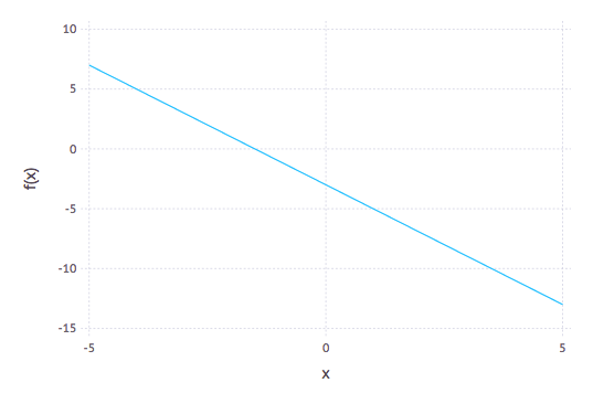
Then $2⊕3=2$ and $3⊗5=8$. To see this in a larger scope, consider the following plots: the function $f(x) = -2x-3$ we get the very nice line:
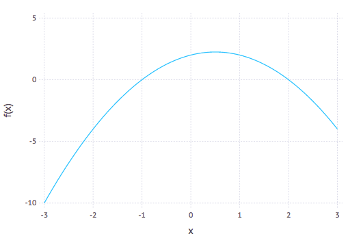
and a plot of the quadratic $y=-x^{2}-x+2$ is
Instead of using what we typically think of as + and $\times$, if we define:
$$x\oplus y = \mbox{min}(x,y)$$
and
$$x \otimes y = x+y $$
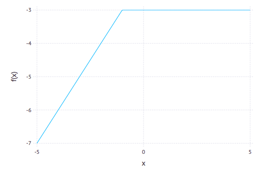
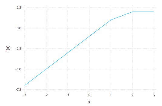
Then using this, we can plot $f(x)=-2\otimes x\oplus(-3)$ and $g(x) = (-1)\otimes x\otimes x \oplus((-1)\otimes x)\oplus 2$
Tropical Matrix Arithemetic
We can also do matrix arithmetic tropically. The $⊕$ goes through the same as it element by elements selects the minimum value of the two. However, tropical matrix multiplication is a little more involved, although it is defined in a very consistent manner. If
$$A = \left[\begin{array}{cc} 2 &4 \newline 5 & 4 \end{array}\right]$$
and
$$
B = \left[\begin{array}{cc} 4 &1 \newline 6 & 6 \end{array}\right]
$$
then
$$ A⊗B = \left[\begin{array}{cc}
\left[\begin{array}{cc}2 & 4 \end{array}\right] ⊗
\left[\begin{array}{c} 4 \newline 6 \end{array}\right] &
\left[\begin{array}{cc}2 & 4 \end{array}\right] ⊗
\left[\begin{array}{c} 1 \newline 6 \end{array}\right] \newline
\left[\begin{array}{cc}5 & 4 \end{array}\right] ⊗
\left[\begin{array}{c} 4 \newline 6 \end{array}\right] &
\left[\begin{array}{cc}5 & 4 \end{array}\right] ⊗
\left[\begin{array}{c} 1 \newline 6 \end{array}\right]
\end{array}\right]$$
$$ A⊗B = \left[\begin{array}{cc}
(2 ⊗ 4)⊕(4⊗6) & (2⊗1)⊕(4⊗6)\newline
(5 ⊗ 4)⊕(4⊗6) & (5⊗1)⊕(4⊗6)\newline
\end{array}\right]
$$
$$ A⊗B = \left[\begin{array}{cc}
6⊕10 & 3 ⊕10 \newline
9 ⊕10 & 6 ⊕10\end{array}\right]
= \left[\begin{array}{cc}
6 & 3 \ 9 & 6
\end{array}\right]
$$
Tropical Math in Julia
Download the TropicalMath package and place it in the local directory. Then load it:
using .TropicalMathThe TropicalMath package exports ⊕ and ⊗ as explained above. For example
3⊕5returns 3 and
2⊗4returns 6. And if we define:
A =  [2  4;
 5  4]
and
B=[ 4  1;
 6  6]
then A⊕B returns
2  1
5  4
which is the smaller value of the two matrices element by element and A⊗B returns
6  3
9  6
as explained above.
Shortest Path problems
Next, let’s look at traveling through a weighted graph, but not necessarily doing a TSP problem. For example, let’s use the following graph:
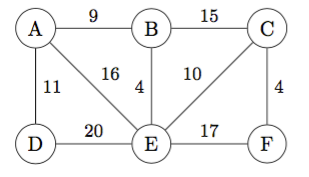
We first create a matrix of the weights:
w=[0 9 Inf 11 16 Inf;
9 0 15 Inf 4 Inf;
Inf 15 0 Inf 10 4;
11 Inf Inf 0 20 Inf;
16 4 10 20 17 0;
Inf Inf 4 Inf 17 0]
where we have include Inf for all paths that don’t have a connection. Note that this becomes a floating-point matrix because the Inf is of type Float64.
This matrix shows the value it costs to travel between any nodes (or $\infty$ if you can’t get from node to another in 1 step.)
For example, it is 15 from B to C.
To find the cost for 2 steps, we calculate the square of the matrix or $A⊗A$.
step2 = w⊗wreturns:
 0.0   9.0  24.0  11.0  13.0  16.0
 9.0   0.0  14.0  20.0   4.0   4.0
24.0  14.0   0.0  30.0  10.0   4.0
11.0  20.0  30.0   0.0  20.0  20.0
13.0   4.0   4.0  20.0   8.0   0.0
33.0  19.0   4.0  37.0  14.0   0.0
which shows the shortest distance between any two nodes. For example, in one step it costs 16 to go from A to E in a single step, but in 2 steps, it costs 13 since A to B then to E is cheaper.
If we look at 3 steps, then
step3 = (w⊗w)⊗wreturns
 0.0   9.0  20.0  11.0  13.0  13.0
 9.0   0.0   8.0  20.0   4.0   4.0
23.0  14.0   0.0  30.0  10.0   4.0
11.0  20.0  24.0   0.0  20.0  20.0
13.0   4.0   4.0  20.0   8.0   0.0
28.0  18.0   4.0  34.0  14.0   0.0
Many of which are the same, but looking at A to C in 2 steps costs 24 which in 3 steps costs 23. (Can you see the path?)
Next, 4 steps results in
step4 = (w⊗w)⊗(w⊗w)which is
0.0   9.0  17.0  11.0  13.0  13.0
9.0   0.0   8.0  20.0   4.0   4.0
23.0  14.0   0.0  30.0  10.0   4.0
11.0  20.0  24.0   0.0  20.0  20.0
13.0   4.0   4.0  20.0   8.0   0.0
27.0  18.0   4.0  34.0  14.0   0.0
and it may appear that this is the matrix but you can check with step3 ≈ step4 or step3-step4 shows the difference in the 5th row, 1st column.
One more step shows:
step4 = (w⊗w)⊗(w⊗w) ⊗ wwhich is
0.0   9.0  17.0  11.0  13.0  13.0
9.0   0.0   8.0  20.0   4.0   4.0
23.0  14.0   0.0  30.0  10.0   4.0
11.0  20.0  24.0   0.0  20.0  20.0
13.0   4.0   4.0  20.0   8.0   0.0
27.0  18.0   4.0  34.0  14.0   0.0
and this hasn’t changed, so we have found the shorted paths between all nodes. For example, the shortest path between node A and F
Dijkstra’s shortest path algorithm
A classic algorithm to solve this problem is called Dijkstra’s Shortest Path Algorithm. Let’s look at the graph from before:
If we want to find the shortest path from node A to node F, first label node A with 0 (as the distance from A) and all other nodes with $\infty$.
- Find all vertices connected to A and label each with the distance to node A
- From each of these nodes, find the distances to unvisited nodes.
- Continue until you pass through the graph. The result will be the shortest distance.
Solving the shortest path problem in Julia using Dijkstra’s algorithm
For this, we will use the LightGraphs and the GraphPlot packages. You will probably need to Pkg.add("LightGraphs") and Pkg.add("GraphPlot") then
using LightGraphs, GraphPlotTo build the graph above and plot it, we will do the following:
G₁ = Graph(6) # graph with 6 vertices

node_info = [
  (1,2,9)
  (1,4,11)
  (1,5,16)
  (2,3,15)
  (2,5,4)
  (3,5,10)
  (3,6,4)
  (4,5,20)
  (5,6,17)
]

wts=zeros(Int,6,6)
for node in node_info
  add_edge!(G₁,node[1],node[2])
  wts[node[1],node[2]] = node[3]
  wts[node[2],node[1]] = node[3]
end

gplot(G₁, nodelabel=["A","B","C","D","E","F"],edgelabel=map(node->node[3],node_info))
which should look similar to:
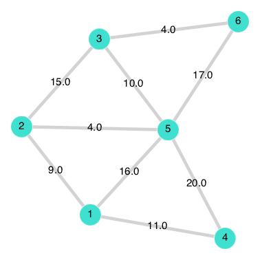
note: each time you run gplot it may look different, so the graph will be the same, but the plot may look rotated or squished.
Finally, we run the following function to find the shortest path (note, the last number is the source vertex):
r = dijkstra_shortest_paths(G₁,1,wts)where the output is pretty unintelligible, however,
r.distsreturns
6-element Array{Float64,1}:
  0.0
  9.0
 23.0
 11.0
 13.0
 27.0
which is the distance of the shortest path from the source vertex (which we said was 1). Since we were looking for the distance to F (or 6), the distance is 27. Also, note that this result is the same as the first row of the matrix returned by the tropical matrix arithmetic above.
To determine the path, using
enumerate_paths(r)
returns the shortest path from the first node to every other node. The last one [1,2,5,3,6] returns the one we want.