Performing LOP Matrix Operations using Software

Section 8.2 Performing LOP Matrix Operations using Software

Objectives

Perform matrix operations in WebCAS.
🔗

🔗
Perform matrix operations (with rational numbers) in Julia.
🔗

🔗

This section covers how to effectively and efficiently perform the matrix operations presented in Section 8.1.

Subsection 8.2.1 Perform the Matrix Operations to Solve LOP problems in WebCAS

WebCAS not only performs row operations on matrices, but also the standard matrix operations. First go to the the Matrix Calculator section of WebCAS. There are two sections of this web page:

🔗

On the right side, there is a place to enter matrices. This is the place to start to enter a matrix or vector with a name. The Matrix Expression textbook is how operations are performed.

🔗

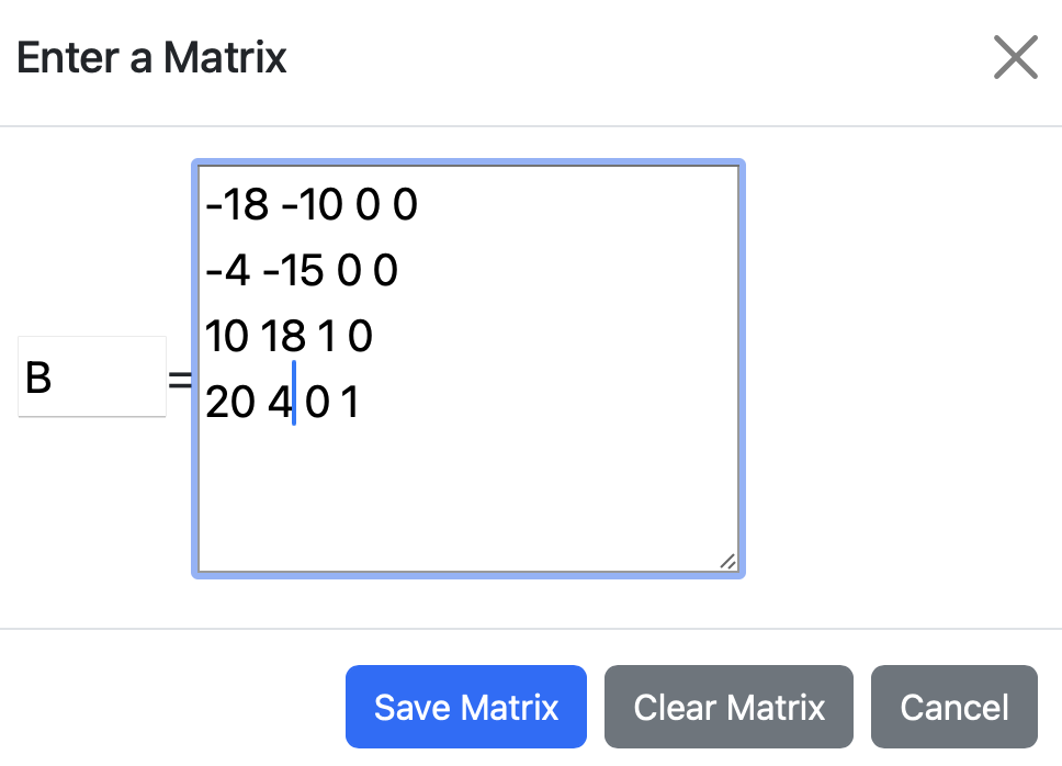
This tool is very general, but we will show the operations from Section 8.1. First, click the Add a new Matrix button and you should see:

🔗

Next, let’s enter the matrix in Example 8.1.3. We first enter the matrix \(B\) with the basis \(\beta=\{1,3,6,7\}\text{.}\)

🔗

where the name of the matrix goes in the left (smaller) textbox and the matrix is entered in the right side in the same manner as that in the Gaussian Eliminator tool. That is, row by row with no commas or other separating characters. Click Save Matrix as you will see it rendered like a matrix in the Matrix Area on the right side. (Note: you can edit the matrix or delete it with the boxes on the right side of it. )

🔗

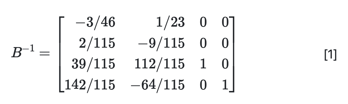
Next, let’s do an operation on B, specifically the inverse using inv(B) by entering this in the Matrix Expression textbook. Either click the Enter button or hit the return key. You will see the inverse as

🔗

Note a few things about this. First, the operation that was performed is shown. That is, \(B^{-1}\text{.}\) Next, the operation using fractions and finally, there is a [1] shown on the right side. We will be able to use this with other operations later.

🔗

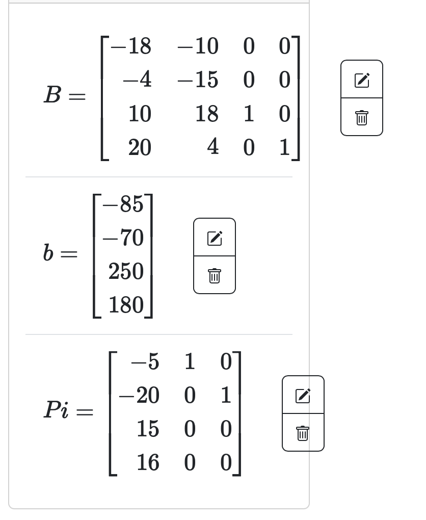
Next, let’s add another vector and matrix. Add \(\boldsymbol{b}\) and \(\Pi\) from Example 8.1.3. For the vector, it is a column vector, so each number should be in a separate row. Also, use the name Pi as that we can’t put Greek letters in for matrix names. You should see:

🔗

Next, to continue with the calculations in Example 8.1.3, to compute \(B^{-1}\boldsymbol{b}\text{,}\) enter [1]*b, where [1] is the output on line 1. The output is the same as seen in Example 8.1.3. Note: the Matrix Operations tool does not perform implicit multiplication, so make sure you specifically enter * for all multiplications.

🔗

To compute \(B^{-1}\Pi\text{,}\) enter [1]*Pi. The result is that seen in Example 8.1.3.

🔗

To finish with the last two steps, first enter \(\boldsymbol{c}_{\beta}\) and \(\boldsymbol{c}_{\pi}\text{.}\) Use the names cbeta and cpi and make sure that each element goes on a separate line.

🔗

To calculate \(\boldsymbol{c}^{\intercal}B^{-1}\boldsymbol{b}\text{,}\) first note that \(B^{-1}\boldsymbol{b}\) has already be computed and is in output [2]. We next need to compute \(\boldsymbol{c}_{\beta}^{\intercal}\text{,}\) which is the transpose of \(\boldsymbol{c}_{\beta}\text{.}\) This is done with cbeta' and returns

🔗

\begin{equation*} {cbeta}^{\intercal} = \left[\begin{array}{cccc} 40 \amp 72 \amp 0 \amp 0\end{array}\right]. \end{equation*}

🔗

and if you have the same steps, this output is now in row [4].

🔗

Now, to compute \(\boldsymbol{c}^{\intercal}B^{-1}\boldsymbol{b}\text{,}\) enter [4]*[2] and you should get

🔗

\begin{equation*} ({cbeta}^{\intercal})((B^{-1}) b) = [388] \end{equation*}

🔗

where the result is a 1 by 1 matrix, which should be interpreted as a scalar.

You probably also notice that there are many unneeded parentheses in the output. It’s a bit tricky to programmatically determine when a set of parentheses is needed.

🔗

Lastly, we also have the expression \(\boldsymbol{c}_{\beta}^{\intercal}B^{-1}\Pi - \boldsymbol{c}_{\pi}^{\intercal}\text{.}\) Some of these already exist, but note that these are all matrices (or actually row vectors) and if we first find \(B^{-1}\Pi\) using [1]*Pi and this returns:

🔗

\begin{equation*} (B^{-1})Pi = \begin{bmatrix} -25/46 \amp -3/46 \amp 1/23 \\ 34/23 \amp 2/115 \amp -9/115 \\ -142/23 \amp 39/115 \amp 112/115 \\ 482/23 \amp 142/115 \amp -64/115 \end{bmatrix} \end{equation*}

🔗

and it’s output is [6]. Next we can find \(\boldsymbol{c}_{\beta}^{\intercal}B^{-1}\Pi\) with [4]*[6] and the output is

🔗

\begin{equation*} ({cbeta}^{\intercal})((B^{-1}) Pi) = \begin{bmatrix} 1948/23 \amp -156/115 \amp -448/115 \end{bmatrix} \end{equation*}

🔗

The next step is to compute \(\boldsymbol{c}_{\pi}^{\intercal}\) with cpi' which returns

🔗

\begin{equation*} cpi^{\intercal} = \begin{bmatrix} 36 \amp 0 \amp 0 \end{bmatrix} \end{equation*}

🔗

in output [8]. Finally we can compute \(\boldsymbol{c}_{\beta}^{\intercal}B^{-1}\Pi - \boldsymbol{c}_{\pi}^{\intercal}\) with [7]-[8]

🔗

and the output in line [9] is

🔗

\begin{equation*} ({cbeta}^{\intercal})((B^{-1}) Pi) - (cpi^{\intercal})= \begin{bmatrix} 1120/23 \amp -156/115 \amp -448/115 \end{bmatrix} \end{equation*}

🔗

Checkpoint 8.2.6.

Complete Example 8.1.4 using WebCAS (Matrix Calculator). Note: det(A) will give you the determinant of the matrix A in WebCAS.

🔗

Subsection 8.2.2 Using Julia to perform Matrix Operations in solving LOP problems.

In the previous section, we used WebCAS to perform the matrix operations from Section 8.1. Although it performed nicely to calculate matrixes with fractions instead of floating point, we needed to break down the steps in order to get it to perform well. Also, as we will see, the same steps are performed with a different basis each time and in WebCAS, the steps will need to be retyped in.

🔗

Alternatively, this section shows how to perform the steps in Julia, which allows some scripting and in the long term is easier to use with some setup.

🔗

If you haven’t yet, review the basics of Julia that you will need in Chapter 5, especially Section 5.3, which discusses handling matrices in Julia.

🔗

To begin with, we will define A, b and c to be the standard coefficient matrix, right-hand side and objective function. In the case of Example 8.1.4 define

🔗

A = [-18 -5 -10
  -4 -20 -15
  10 15 18
  20 16 4]
b = [-85, -70, 250, 180]
c = [40, 36, 72]

Recall that \(B\) and \(\Pi\) are defined by the basis and the parameter set. It will actually help quite a bit to define these as

🔗

β = [1,3,6,7]

where you can create β with \beta and then hit tab (in a julia notebook). The parameters, π, is the variables not in the basis which can be generated with

🔗

π = setdiff(collect(1:7), β)

where the collect(1:7) generates the vector of all integers between 1 and 7. The setdiff function will return all the numbers between 1 and 7 that are not in β.

🔗

B = rationalize.(hcat(A, I)[:, β])
Π = hcat(A, I)[:, π]

where the hcat function performs a horizontal concatenation between \(A\) and the identity matrix. The [:,β] returns only the columns in β and simiilarly for π. The rationalize function takes each integer and converts it to a rational number. This is helpful for creating an inverse that is rational and the . is for broadcasting, but the matrix Π is never inverted, so we don’t need to use rationalize. If both commands are in a single cell, only the last one will be echoed to the screen or

🔗

4×3 Matrix{Rational{Int64}}:
  -5  1  0
 -20  0  1
  15  0  0
  16  0  0

🔗

Lastly, we will also redefine \(c\) to be

🔗

c = [40, 36, 72, 0, 0, 0, 0]

Then you can get \(c_{\beta}\) in julia using c[β] and the result is

🔗

4-element Vector{Int64}:
 40
 72
  0
  0

🔗

Now that all of the parts have been defined, repeating Example 8.1.4 is quite straightforward.

🔗

To find \(B^{-1}\text{,}\) use inv(B) and the result is
🔗
```
4×4 Matrix{Rational{Int64}}:
  -3//46     1//23   0  0
   2//115   -9//115  0  0
  39//115  112//115  1  0
 142//115  -64//115  0  1
```
🔗
and this is the same that we got using WebCAS. Note that a rational number in Julia has a //.
🔗

🔗
To get \(B^{-1}\boldsymbol{b}\text{,}\) enter inv(B)*b and the result is
🔗
```
4-element Vector{Rational{Int64}}:
  5//2
   4
 153
 114
```
🔗
and this is the same as above as well as in the exercise.
🔗

🔗

To find \(B^{-1}\Pi\) enter inv(B)*Π and the result is

🔗

4×3 Matrix{Rational{Int64}}:
  -25//46   -3//46     1//23
   34//23    2//115   -9//115
 -142//23   39//115  112//115
  482//23  142//115  -64//115

🔗

To find \(\boldsymbol{c}_{\beta}^{\intercal}B^{-1}\boldsymbol{b}\text{,}\) enter c[β]'*inv(B)*b and it returns 388//1, which is the rational (fraction) version of 388, which we found above.
🔗

🔗
Lastly, to find \(\boldsymbol{c}_{\beta}^{\intercal}B^{-1}\Pi - \boldsymbol{c}_{\pi}^{\intercal}\) enter c[β]'*inv(B)*Π-c[π]' to get
🔗
```
1×3 adjoint(::Vector{Rational{Int64}}) with eltype Rational{Int64}:
 1120//23  -156//115  -448//115
```
🔗
which is a bit complicated (it’s saying it is an adjoint, which is a general transpose). The important thing is that it is a row vector of length 3 and the same that we got above and in the exercise.
🔗

🔗

🔗

Checkpoint 8.2.7.

Use Julia to evaluate all of the expressions in Example 8.1.4 and note that the determinant in Julia is det.

🔗

(a)

\(d_{\beta}\)

🔗

Solution.

using dβ = det(B) and the result is 230//1 a rational version of the determinant. Instead, we will use dβ = round(Int, det(B)) or 230.

🔗

(b)

\(B'\)

🔗

Solution.

Similar to the previous one, this should be an integer matrix, so if we do

🔗

Bp = round.(Int, dβ * inv(B))

and this returns:

🔗

4×4 Matrix{Int64}:
 -15    10    0    0
   4   -18    0    0
  78   224  230    0
 284  -128    0  230

🔗

(c)

\(B'\boldsymbol{b}\)

🔗

Solution.

If we do Bp*b, the result is

🔗

4-element Vector{Int64}:
   575
   920
 35190
 26220

🔗

(d)

\(B'\Pi\)

🔗

Solution.

Performing Bp*Π results in

🔗

4×3 Matrix{Rational{Int64}}:
  -125  -15    10
   340    4   -18
 -1420   78   224
  4820  284  -128

🔗

(e)

\(\boldsymbol{c}_{\beta}^{\intercal} B' \boldsymbol{b}\)

🔗

Solution.

Enetering c[β]'*Bp*b results in 89240.

🔗

(f)

\(\boldsymbol{c}_{\beta}^{\intercal} B' \Pi - d_{\beta} \boldsymbol{c}_{\pi}^{\intercal} \)

🔗

Solution.

Entering c[β]'*Bp*Π - dβ *c[π]' results in

🔗

1×3 adjoint(::Vector{Int64}) with eltype Int64:
11200  -312  -896

🔗

Prev Top Next