Advanced Topics in Linear Algebra

Chapter 41 Advanced Topics in Linear Algebra

We just dipped our toes into the land of Linear Algebra in the previous chapter. There are many other topics. This covers some of them.

🔗

Section 41.1 Newton’s method for more than one variable

We saw Newton’s method in Section 10.4

🔗

As an example that we might be interested in is to solve multiple equations for multiple variables. Let’s find the intersection between the line \(y=x+1\) and the circle \(x^2+y^2=25\text{.}\) A plot of this situation is

🔗

Recall that for a function of one variable, Newton’s method is used to find a root of an equation, that is, a number \(x^{\star}\) such that \(f(x^{\star}) = 0\text{.}\) We are going to extend this to two functions of two variables. We seek numbers \((x^{\star}, y^{\star})\) such that \(f(x^{\star},y^{\star}) = 0\) and \(g(x^{\star},y^{\star})=0\text{.}\) In the picture above, there are two such pairs of numbers where the two curve intersect.

🔗

To derive Newton’s method for this situation, we’ll switch some notation. First, let \(\vec{F}(\vec{x}) = \langle f(x,y), g(x,y) \rangle\) be the vector function from \(\mathbb{R}^2\) to \(\mathbb{R}^2\text{.}\) We use the Taylor Expansion (REF???) at some point \(\vec{x}\) near the root \(\vec{x}^{\star}\) as

🔗

\begin{equation*} \vec{F}(\vec{x}^{\star}) = \vec{F}(\vec{x}) + J(\vec{x}) (\vec{x}^{\star}-\vec{x}) + O(||\vec{x}^{\star} -\vec{x}||^2) \end{equation*}

🔗

where \(J\) is the Jacobian matrix given by

🔗

\begin{equation} J = \begin{bmatrix} \frac{\partial f}{\partial x} \amp \frac{\partial f}{\partial y} \\ \frac{\partial g}{\partial x} \amp \frac{\partial g}{\partial y} \end{bmatrix}\tag{41.1} \end{equation}

🔗

If we linearize this by dropping the \(O(||\vec{x}^{\star}-\vec{x}||)\) term and note that \(\vec{F}(\vec{x}^{\star}) = \vec{0} \) because it is a root, then the result is the linear system:

🔗

\begin{equation*} \vec{F}(\vec{x}) = - J(\vec{x}^{\star} - \vec{x}) \end{equation*}

🔗

This is now used for Newton’s method. Above, let \(\vec{x} = \vec{x}_n\) and then we’ll estimate \(\vec{x}_{n+1} = \vec{x}^{\star}\text{.}\) Also, for convience, we’ll define \(\vec{\Delta}_{n+1} = \vec{x}_{n+1} - \vec{x}_n\text{.}\) Thus Newton’s method turns into

🔗

\begin{align} J \vec{\Delta}_{n+1} \amp = - \vec{F}(\vec{x}_n) \qquad \text{Solve for \(\vec{\Delta}_{n+1}\)}\tag{41.2}\\ \vec{x}_{n+1} \amp = \vec{x}_n + \vec{\Delta}_{n+1}\tag{41.3} \end{align}

🔗

Although we derived this for two functions with two variables each, the above analysis works for vector functions from \(\mathbb{R}^n\)to \(\mathbb{R}^n\text{.}\) The Jacobian matrix shown in (41.1) can be extended as an \(n \times n\) matrix and the Newton method in (41.2) and (41.3) works in general.

🔗

Subsection 41.1.1 Implementing Newton’s Method for Multidimensions

Now we turn to implementing this. Although it will be very similar to the 1D Newton’s method that we developed in Section 10.4, there are some differences here, mainly in that the first step of Newton’s method in (41.2) is a matrix equation and has the form \(A \vec{x} = \vec{b}\) that we solved in Section 40.3.

🔗

function newton(F::Function, x0::Vector{<:Real}; max_steps::Int = 20, eps::Real = 1e-6)
  for _ = 1:max_steps
    Δ = -ForwardDiff.jacobian(F,x0) \ F(x0)
    norm(Δ) < eps && return x0
    x0 += Δ
  end
  error("Newton's method didn't converge in $max_steps steps.")
end

First, notice that this looks much like the same structure as the 1D Newton’s method. There are two differences. First, we use one line 3 the jacobian method that is in the ForwardDiff package. This calcuates the Jacobian matrix that we saw in (41.1) if we are given a point. Also on line 3, we use the \ to do a linear solve. We used this in Section 40.3. This gave us the value of Δ.

🔗

Line 4 then checks if the norm (square root of the sum of the squares) is small and if so returns the given point. If not, update and repeat. Note that on line 7 that if we got through the for loop without returning, then it didn’t converge and we return an error.

🔗

Example 41.2.

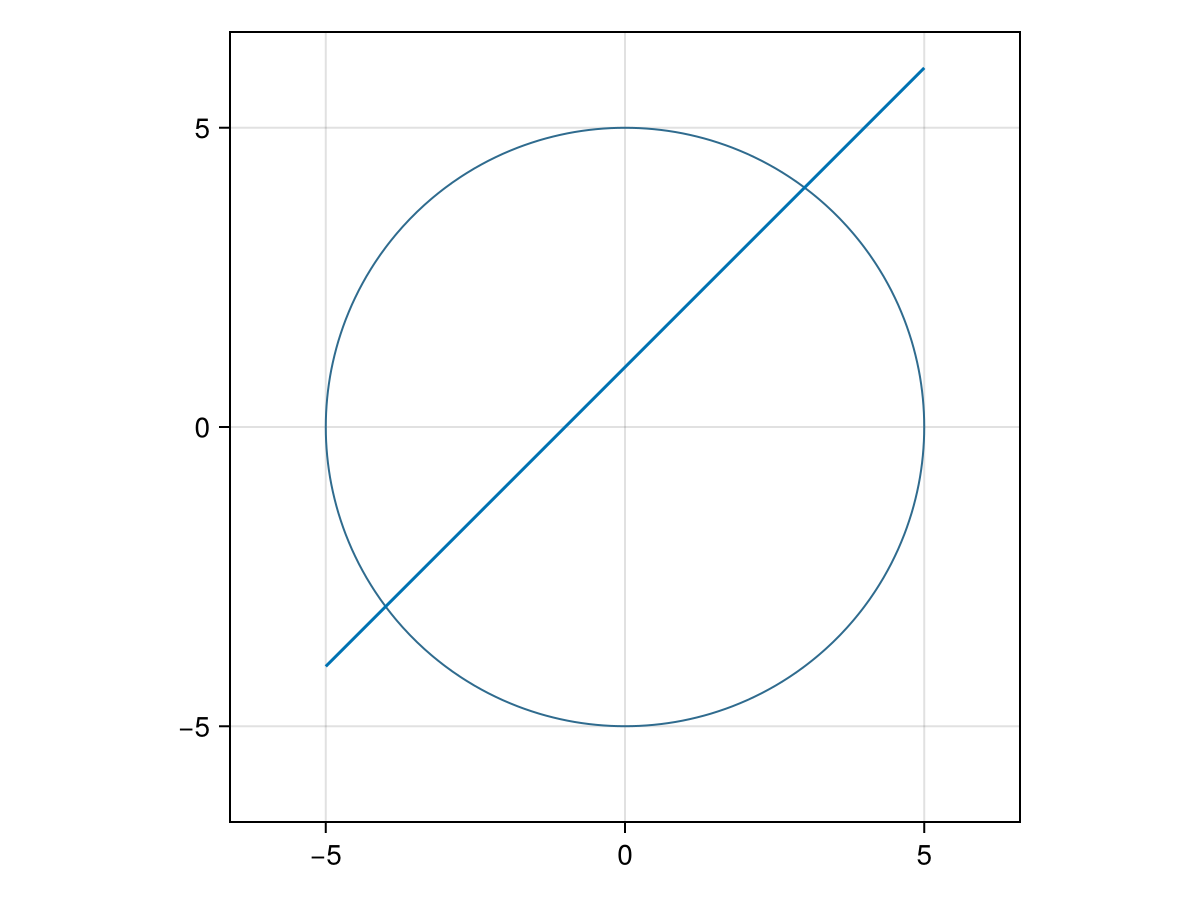
Let’s run Newton’s method on the function. To do this, we will build the function \(\vec{F}(\vec{x})\) using Julia notation. The equations \(y=x+1\) and \(x^2+y^2=25\) can be combined as the function

🔗

F(x::Vector{<:Real}) = [x[1]^2+x[2]^2-25, x[1]-x[2]+1]

🔗

where note that the argument x has been declared as a Real vector and that the first argument is the circle and the second is the line. Notice that the variables \(x\) and \(y\) are encoded as x[1] and x[2]

🔗

Running Newton’s method at the point \((1,1)\) is accomplished with newton(F,[1,1]) and results in

🔗

2-element Vector{Float64}:
 3.0000000730550047
 4.000000073055005

🔗

which finds the point \((3,4)\) to within the default \(10^{-6}\text{.}\) If we start with the initial point [-1,-1] the point \((-3,-4)\) is found.

🔗

Check Your Understanding 41.3.

Find a solution to the equations

🔗

\begin{align*} 36x^2+9y^2+4z^2 \amp =72 \amp z^2-x^2 \amp = 6 \amp 2x + 3y \amp =4 \end{align*}

🔗

Subsection 41.1.2 Problems that can occur for Newton’s method

We saw cases where 1D Newton’s method ran in problems. This was usually when the derivative was 0 at an inital (or subsequent) point. This can occur in this situation as well, but even moreso.

🔗

For example, returning to Example 41.2 let’s consider if we select the point to start at as \((1,-1)\text{.}\) If we run newton(F,[1,-1]), then we get an error: SingularException(2).

🔗

To explore what’s going on, update newton’s method to

🔗

function newton(F::Function, x0::Vector{<:Real}; max_steps::Int = 20, eps::Real = 1e-6)
  for _ = 1:max_steps
    J = ForwardDiff.jacobian(F, x0)
    @show J
    @show det(J)
    Δ = -J \ F(x0)
    norm(Δ) < eps && return x0
    x0 += Δ
  end
  error("Newton's method didn't converge in $max_steps steps.")
end

Rerunning now with newton(F,[1,-1]) results in

🔗

J = [2 -2; 1 -1]
det(J) = 0.0
SingularException(2)

🔗

Notice that the matrix J has rows that are multiples of each other which results in a 0 determinant means that the matrix is Singular.

🔗

Although this can happen, generally changing an initial point can help with this. However, let’s add some information when this happens and update newton’s method to

🔗

function newton(F::Function, x0::Vector{lt;:Real}; max_steps::Int = 20, eps::Real = 1e-6)
  for _ = 1:max_steps
    J = ForwardDiff.jacobian(F,x0)
    det(J) ≈ 0 && error("Newton's method reached a singular point of the Jacobian.")
    Δ = - J \ F(x0)
    norm(Δ) < eps && return x0
    x0 += Δ
    @show x0
  end
  error("Newton's method didn't converge in $max_steps steps.")
end

🔗

Section 41.2 Sparse Matrices

We saw in the previous chapter, some of the matrices contained many zeros. As matrices get larger, the structure of them (like banded matrices), results in a matrix that is almost all zeros.

🔗

Consider the matrix:

🔗

A = [
  0   1    0    0    0    0   0   0   0   0   0   0   0 ;
  0   0    0    0    0    2   0   0   0   0   0   0   0 ;
  0   0   -1    0    0    0   0   0   0   0   0   0   0 ;
  0   0    0    0    0    0   0   0   0   1   0   0   0 ;
  0   0    0    0   -2    0   0   0   0   0   0   0   0 ;
  1   0    0    0    0    0   0   0   0   0   0   0   0 ;
  0   0    0    0    0    0   0   0   0   0   0   0  -1 ;
  0   0    0    0    0    0   2   0   0   0   0   0   0 ;
  0   0    0   -1    0    0   0   0   0   0   0   0   0 ;
  0   0    0    0    0   -2   0   0   0   0   0   0   0 ;
  0   0    0    0    0    0   0   0   0   0   0   1   0 ;
  0   0    0    0    0    0   0   0   0   0   2   0   0 ;
  0   0    0    0    0    0   0   0   1   0   0   0   0 ]

🔗

and there is no apparent structure to the nonzero elements. Although this isn’t that large, imagine a 1000 by 1000 version of this array with 1% of the elements nonzero. If we used a regular matrix, then such a matrix would take \(1000^2 \cdot 8\) bytes, which is quite large. We can see this with sizeof(A) which returns 1352, which is \(13^2 \cdot 8\text{.}\)

🔗

Instead, we will use a SparseMatrixCSC in the SparseArrays package to store these. There are a couple of ways to create the matrix. If it is stored as a regular (dense) matrix, then it can be converted easily.

🔗

using SparseArrays
SA = SparseMatrixCSC(A)

🔗

which returns

🔗

13×13 SparseMatrixCSC{Int64, Int64} with 13 stored entries:
  ⋅  1   ⋅   ⋅   ⋅   ⋅  ⋅  ⋅  ⋅  ⋅  ⋅  ⋅   ⋅
  ⋅  ⋅   ⋅   ⋅   ⋅   2  ⋅  ⋅  ⋅  ⋅  ⋅  ⋅   ⋅
  ⋅  ⋅  -1   ⋅   ⋅   ⋅  ⋅  ⋅  ⋅  ⋅  ⋅  ⋅   ⋅
  ⋅  ⋅   ⋅   ⋅   ⋅   ⋅  ⋅  ⋅  ⋅  1  ⋅  ⋅   ⋅
  ⋅  ⋅   ⋅   ⋅  -2   ⋅  ⋅  ⋅  ⋅  ⋅  ⋅  ⋅   ⋅
  1  ⋅   ⋅   ⋅   ⋅   ⋅  ⋅  ⋅  ⋅  ⋅  ⋅  ⋅   ⋅
  ⋅  ⋅   ⋅   ⋅   ⋅   ⋅  ⋅  ⋅  ⋅  ⋅  ⋅  ⋅  -1
  ⋅  ⋅   ⋅   ⋅   ⋅   ⋅  2  ⋅  ⋅  ⋅  ⋅  ⋅   ⋅
  ⋅  ⋅   ⋅  -1   ⋅   ⋅  ⋅  ⋅  ⋅  ⋅  ⋅  ⋅   ⋅
  ⋅  ⋅   ⋅   ⋅   ⋅  -2  ⋅  ⋅  ⋅  ⋅  ⋅  ⋅   ⋅
  ⋅  ⋅   ⋅   ⋅   ⋅   ⋅  ⋅  ⋅  ⋅  ⋅  ⋅  1   ⋅
  ⋅  ⋅   ⋅   ⋅   ⋅   ⋅  ⋅  ⋅  ⋅  ⋅  2  ⋅   ⋅
  ⋅  ⋅   ⋅   ⋅   ⋅   ⋅  ⋅  ⋅  1  ⋅  ⋅  ⋅   ⋅

🔗

Notice that it only stores the nonzero elements. To determine that the storage amount is indeed small, entering sizeof(SA) which returns 40.

🔗

Let’s create a sparse vector with the following command:

🔗

R = sparsevec([1,5,7,12,13],[-1,5,10,3,5])

🔗

which returns

🔗

13-element SparseVector{Int64, Int64} with 5 stored entries:
  [1 ]  =  -1
  [5 ]  =  5
  [7 ]  =  10
  [12]  =  3
  [13]  =  5

🔗

and notice that lists the elements of the vector that are nonzero.

🔗

Note: This section needs to be filled out a bit.

🔗

Prev Top Next