
Chapter 28 Algorithm Analysis

This chapter will be a brief introduction to the analysis of algorithms. As we have already seen in the past couple of chapters, timing algorithms is a decent way to determining how well they run, however sometimes a more in-depth analysis is needed. We will cover what is called big-O notation and analyze a few algorithms here.

Section 28.1 Big-O Notation

Definition 28.1.

Consider two functions \(f\) and \(g\text{,}\) We say that \(f(n)\) is \(O(g(n))\) or ``big-O’’ of \(g(n)\) if
\begin{equation*} \lim_{n \rightarrow \infty} \frac{f(n)}{g(n)} = C \end{equation*}
for some \(0 > C > \infty\text{.}\)
For example, let \(f(n) = 3n^2-2n+6\text{.}\) This function is \(O(n^2)\) because
\begin{equation*} \lim_{n\rightarrow \infty} \frac{3n^2-2n+6}{n^2} = 3 \end{equation*}
Generally, if a function is polynomial, the function is \(O(n^p)\) where \(p\) is the degree of polynomial.

Check Your Understanding 28.2.

For each of the following functions find \(O(g(n))\text{,}\) that is find \(g(n)\text{:}\)
(a)
\(f(n) = n^2+e^n\)
Hint.
Hint: recall L’Hopital’s rule for derivatives and try to find the largest term of the given function.

Section 28.2 Polynomial Evaluation

An example that we will see again in Chapter 12, it that of evaluating a polynomial. If
\begin{equation} p(x) = a_0 + a_1 x + a_2 x^2 + \cdots + a_n x^n\tag{28.1} \end{equation}
If we evaluate the polynomial as is counting powers as repeated multiplication, then the number of additions is \(n\) and the number of multiplication is
\begin{equation*} M(n) = 1 + 2 + 3 + \cdots + n = \frac{n(n+1)}{2} \end{equation*}
This shows that polynomial evaluation is \(O(n^2)\) since \(\lim_{n \rightarrow \infty} M(n)/n^2 = 1/2\text{.}\)

Subsection 28.2.1 Horner’s Form

We can rewrite (28.1) as
\begin{equation} p(x) = a_0 + x(a_1 + x(a_2 + x(a_3 \cdots + a_n x)))\tag{28.2} \end{equation}
In this case, there are \(n\) additions and \(n\) multiplications. So you could say that the total number of operations are \(c_1 n + c_2n\) where \(c_1\) and \(c_2\) are constants related to addition and multiplication. Overall, this means that the order of polynomial evaluation using Horner’s method is \(O(n)\text{.}\)

Subsection 28.2.2 Benchmarking Polynomial Evaluation

Let’s actually see some actual data in this. First, the polynomial evaluation can be written as
function poly1(coeffs::Vector{T}, x::S) where {T <: Number, S <: Number}
  local sum = zero(T)
  function pow(x::T,n::Int) where T <: Number
    local prod = one(T)
    for j=1:n
      prod *=x
    end
    prod
  end
  for n=1:length(coeffs)
    sum += coeffs[n]*pow(x,n-1)
  end
  sum
end
where the where {T <: Number, S <: Number} will be explained in Chapter 11, but this allows any subtype of Number to be taken. Also, we have defined the power to be repeated multiplication using a for loop, since Julia’s power function is quite efficient--we want to show the results from above.
To test this, first we will use BigFloats as the coefficients to slow down the operations a bit, otherwise it is hard to measure the time.
Let’s do some testing and we’ll need the BenchmarkTools and CairoMakie (for plotting). We also need Random to set the seed and LsqFit to fit the data we’ll generate to a curve.
using BenchmarkTools, CairoMakie, Random, LsqFit
CairoMakie.activate!()
Random.seed!(132)
Remark 28.3.
There are a few plots in this section and we will be using a package called Makie to do the plots. We will explore this in detail in Chapter 14, however, copying the code to produce the plots is sufficient for this chapter.
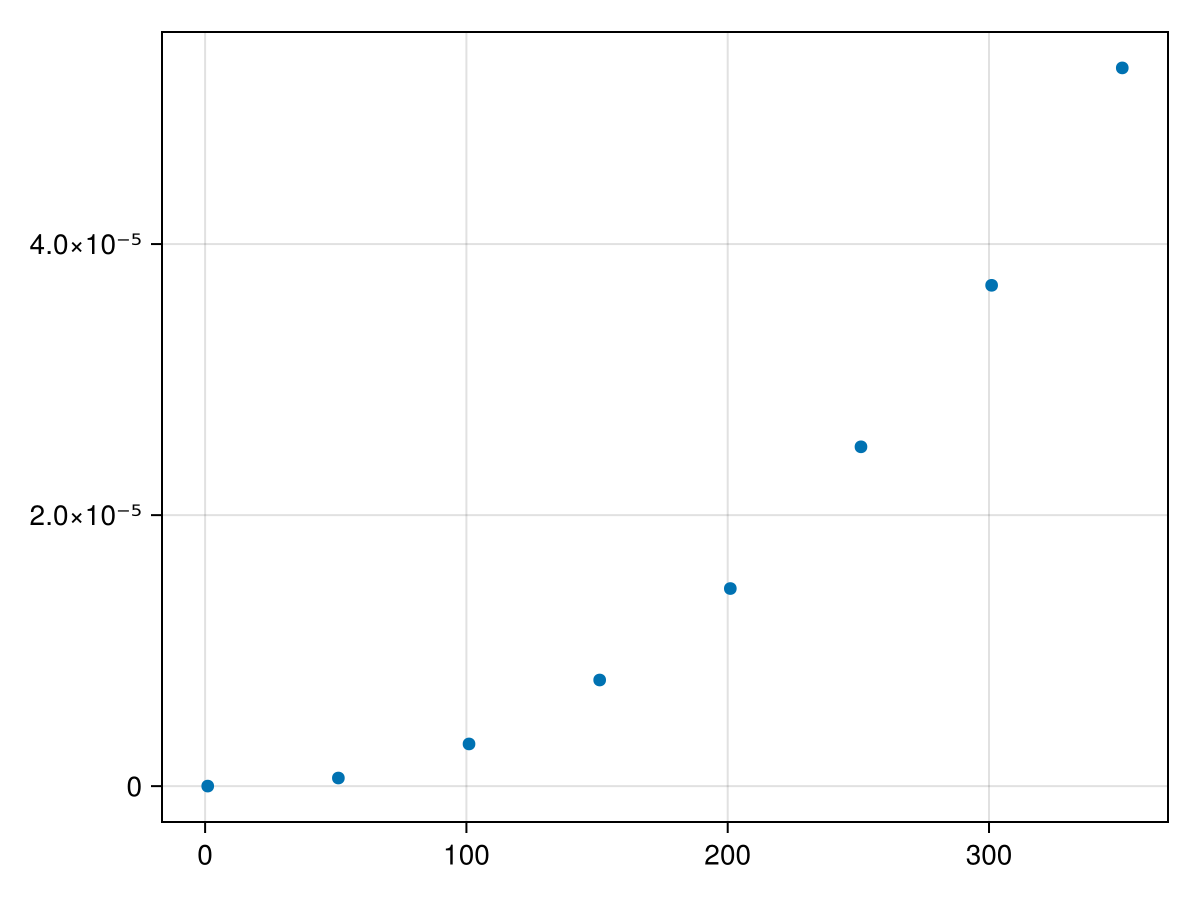
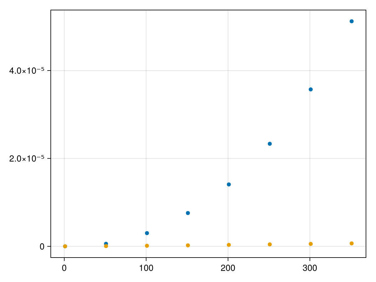
The following will time using the @belapsed macro which returns the amount of time a function takes given in seconds. This is needed because we need to store the result. Note that in the previous chapters we’ve used the @btime macro which times the function and gives additional information as well as the return value. We are only interested in the amount of time in this section.
time = zeros(351)
r = 1:50:351
for i=r
  coeffs = rand(i+1)
  time[i] = @belapsed poly1($coeffs,1/3)
end
which will take quite a bit time. After this runs, if we create a scatter plot with
fig, ax = scatter(r,time[r])
(for accessibility)
Figure 28.4.
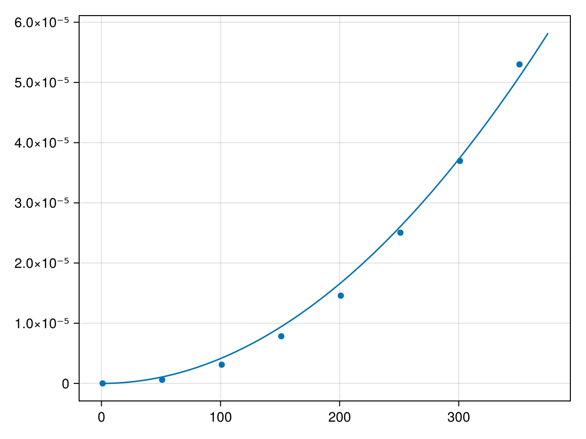
Hopefully visually you can see that it appears to be nonlinear and perhaps you can see that it is may be quadratic. We will fit a quadratic to these points by first defining the model as a quadratic:
model(t, p) = @. p[1]+p[2]*t+p[3]*t^2
where broadcasting using @. that was explained in Section 6.5 and then fit the data to the model with:
fit = curve_fit(model, r, time[r], [1e-8,1e-8,1e-8])
and note that the output will not be particularly helpful. What we are looking for are the best-fit parameters and these can be found with fit.param and the results are
3-element Vector{Float64}:
  6.636565666123923e-7
 -3.7652064597589e-8
  6.108561075647983e-10
These are all small, however, the important thing to determine is if they are possibly zero. We can use the confidence interval of each is found with confidence_interval(fit, 0.05) which returns
3-element Vector{Tuple{Float64, Float64}}:
  (-8.762753517690063e-7, 2.203588484993791e-6)
  (-5.8097027280678223e-8, -1.7207101914499782e-8)
  (5.549847084532201e-10, 6.667275066763765e-10)
These show the 95%-confidence intervals for the three parameters. We are looking for the largest non-zero term, which is the third one. Since the above fits all three terms, we will redo the fit with only the third term as
model2(t,p) = @. p[1]*t^2
and then fit the data with
fit2 = curve_fit(model2, r, time[r], [1.0])
We can add the curve to the plot above with:
lines!(ax, 0:225,t->fit2.param[1]*t^2)
which is the following plot
(for accessibility)
Figure 28.5.
and although it doesn’t look like a perfect fit, it does appear to be quadratic.
Subsubsection 28.2.2.1 Horner’s Form
We will compare this to Horner’s form, which we can write in Julia as:
function horner(coeffs::Vector{T},x::S) where {T <: Number, S <: Number}
  local result = coeffs[end]
  for i=length(coeffs)-1:-1:1
    result = x*result+coeffs[i]
  end
  result
end
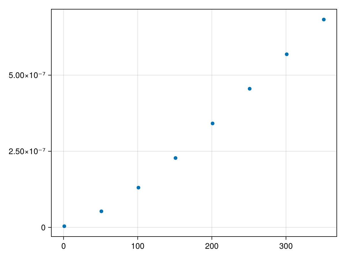
and then similar to above, we will time this method for different lengths:
htime = zeros(351)
r = 1:50:351
for i=r
  coeffs = rand(i)
  htime[i] = @belapsed horner($coeffs,10/3)
end
and plot the results:
scatter(r,htime[r])
which results in
(for accessibility)
Figure 28.6.
and this look much more linear than the previous one. For this model, we’ll fit a linear function.
fit3 = curve_fit((t,p) -> p[1].*t, r, htime[r], [1e-8])
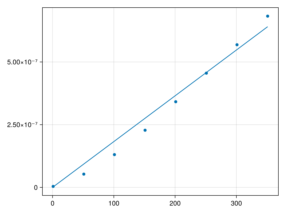
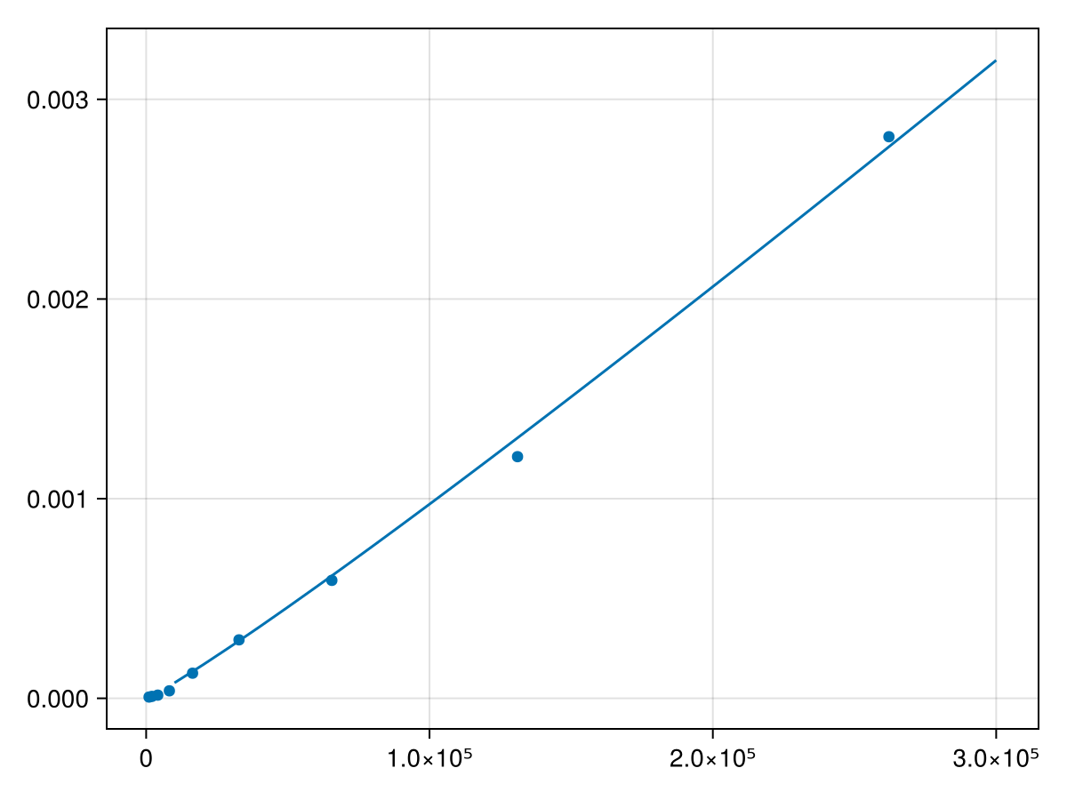
and if you’re interested in the value of the parameter (slope of the line), fit3.param returns 1.8253874361922209e-9. Looking at it visually, let’s add the plot of the line to the scatter plot above with
lines!(ax, 1:360, t->fit3.params[1]*t)
and this results in the following plot:
(for accessibility)
Figure 28.7.
Overall, these results show that the time taken to evaluate a polynomial using Horner’s form, is \(O(n)\text{.}\) This evidence shows that Horner’s form of the polynomial is much faster and putting these two scatter plots together with:
fig, ax =  scatter(r, time[r])
scatter!(ax, r, htime[r])
fig
and the results are
(for accessibility)
Figure 28.8.

Section 28.3 Interpreting big-O results

Typically algorithms grows as some function of \(n\text{,}\) which is a measure of the size of the problem. Determining the order of the algorithm can be tricky although we can use numerics like above to find the timing of algorithms for various sizes of the problem. Then doing some data-fitting, we can often find the order of the algorithm. We’ll see another example of this in the next section.
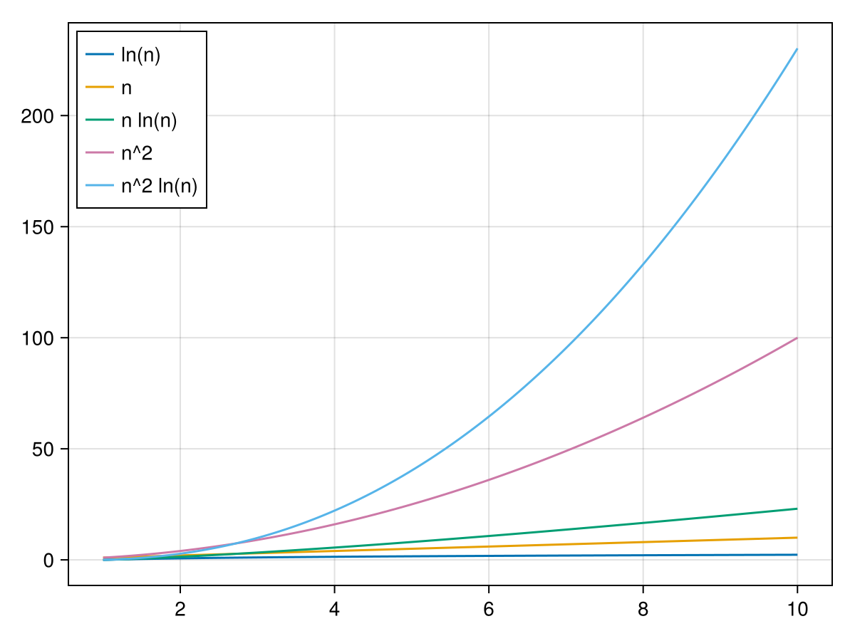
Understanding different orders is helpful and this means understanding how functions grow. Here are a bunch of standard algorithm functions and their plots:
fig = Figure()
ax = Axis(fig[1,1])
pl1 = lines!(ax, 1:0.05:10, x->log(x))
pl2 = lines!(ax, 1:0.05:10, x->x)
pl3 = lines!(ax, 1:0.05:10, x->x*log(x))
pl4 = lines!(ax, 1:0.05:10, x->x^2)
pl5 = lines!(ax, 1:0.05:10, x->x^2*log(x))
axislegend(ax,
  [pl1,pl2,pl3,pl4,pl5],
  ["ln(n)","n","n ln(n)","n^2","n^2 ln(n)"],
  position = :lt
)
fig
And the result is
(for accessibility)
Figure 28.9.
This would basically show that if there are choices of algorithms, to use an algorithm with a lower order in that for large values of problem size will run faster.

Section 28.4 Using Data to determine Algorithm order

Typically, the best way to analyze an algorithm is to determine the number of operations as a function of \(n\text{,}\) however, let’s look at this as a data analysis problem. As an example, we’ll look at this as the Fast Fourier Transform, discussed in Chapter \ref{ch:complex}. This is a classic example of improving an algorithm to change the order. For this we need the FFTW package, which you probably need to add and
 using FFTW 
Let’s first build up a set of times similar to above with
times3 = Float64[]
sizes3 = [2^n for n=10:18]
for size in sizes3
  x=rand(size)
  t = @belapsed fft($x)
  push!(times3,t)
end
which calculates the FFT for sizes 2^10 to 2^18 and stores the results in the variable times. Then, let’s plot the results with
scatter(sizes3,times3, legend = false)
which results in the plot
(for accessibility)
Figure 28.10.
Since it appears to be growing more that linearly, let’s try the functions t*log(t) and t^2. Fitting a curve to both of these is
fit_fft = curve_fit((t,p) -> p[1].*t.*log.(t)+p[2].*t.^2,sizes3, times3, [1e-4,1e-4])
and a confidence interval of the parameters are found with confidence_interval(fit_fft) resulting in
2-element Vector{Tuple{Float64, Float64}}:
  (6.879894218252294e-10, 7.990430330357398e-10)
  (2.557195884568105e-15, 8.361319348915151e-15)
Although both are exclusively positive, the second interval is nearly zero--values near \(10^{-15}\) are often actually 0 and just due to roundoff error. Therefore, we will only use the first term in the model or \(t*log(t)\text{.}\) Trying a new function fit with
fit_fft2 = curve_fit((t,p) -> @. p[1]*t*log(t), sizes3, times3, [1e-4]) 
The confidence interval of the parameters is found with confidence_interval(fit3) and the results are
1-element Vector{Tuple{Float64, Float64}}: (8.197426904649365e-10, 8.695061786080083e-10)
Lastly, we plot the data and the best fit function found above with
fig, ax = scatter(sizes3, times3)
lines!(ax, 0:10^4:3*10^5, x->fit_fft2.param[1]*x*log(x))
fig
plot!(t->fit3.param[1]*t*log(t),first(sizes3),last(sizes3))
And the resulting plot is:
Figure 28.11. Find a point on a line that minimizes distance
This shows using some data analysis that the FFT is \(O(n \ln n)\text{,}\) which can also be shown use analysis of the algorithm, but requires knowledge of how the algorithm works.