Calculating the digits of \pi

Chapter 48 Calculating the digits of \(\pi\)

In Section 19.5, we saw a method to find the digits of \(\pi\) using random numbers. You should have noticed that it was not a very good method in that it took a million or so random numbers to produce 3 digits of \(\pi\text{.}\) In this chapter, we will explore ways to do it using Power Series, a way of representing functions using calculus.

🔗

Recall that a power series is a function of the form:

🔗

\begin{equation*} a_0+a_1 x + a_2 x^2 + \cdots = \sum_{n=0}^{\infty} a_n x^n \end{equation*}

🔗

which is the sum of terms with nonnegative integer powers of \(x\) and an important aspect is that power series do not have a highest power. Nearly every function can be represented by a power series. The classic one is

🔗

\begin{equation} \frac{1}{1-x} = 1+x+x^2+x^3 + \cdots\tag{48.1} \end{equation}

🔗

which is called the geometric series.

🔗

Section 48.1 Power Series of Arctangent

We will see that the arctangent function and resulting power series can produce the digits of \(\pi\) to many digits. Let’s dive into the power series of arctangent.

🔗

If we let \(u=-x^2\) in (48.1), then

🔗

\begin{align*} \frac{1}{1+u^2} \amp = 1+(-u^2) +(-u^2)^2 + (-u^2)^3 + \cdots \\ \amp = 1-u^2 + u^4 - u^6 + \cdots \end{align*}

🔗

Since the variable name doesn’t matter, we can also write this in \(x\) as:

🔗

\begin{equation*} \frac{1}{1+x^2} = 1-x^2+x^4-x^6 + \cdots \end{equation*}

🔗

If we integrate both sides:

\begin{align} \int \frac{1}{1+x^2}\, dx \amp = \int (1-x^2+x^4-x^6 + \cdots ) \, dx \notag\\ \tan^{-1} x \amp = x -\frac{x^3}{3} + \frac{x^5}{5} - \frac{x^7}{7} + \cdots \tag{48.2} \end{align}

🔗

and there is an integration constant, but it is 0, so we haven’t shown it.

🔗

Now we can use the fact that \(\tan^{-1} (1) = \pi/4\text{,}\) so if substitute \(x=1\) into (48.2), then

🔗

\begin{equation*} \frac{\pi}{4} = 1 - \frac{1}{3} + \frac{1}{5} - \frac{1}{7} + \cdots \end{equation*}

🔗

and multiplying through by 4 results in a power series representation of \(\pi\) or

🔗

\begin{equation*} \pi = 4\biggl(1 - \frac{1}{3} + \frac{1}{5} - \frac{1}{7} + \cdots \biggr) \end{equation*}

🔗

We can estimate \(\pi\) using a few terms of the above series in julia with:

🔗

 4*(1-1/3+1/5-1/7+1/9-1/11+1/13-1/15+1/17-1/19)

🔗

and the results are 3.0418396189294032, which hopefully you can tell is not so great. Let’s be more systematic about this though.

🔗

function calcPi(n::Integer)
  n > 0 || throw(ArgumentError("The input n must be positive."))
  local sum = 1.0
  for k=1:n
    sum += (-1)^k/(2k+1)
  end
  4*sum
end

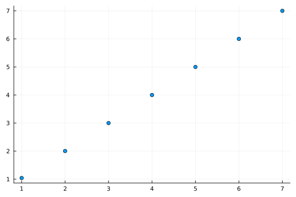
for example, we can now determine 10,000 terms of this series with

🔗

pi10_000 = calcPi(10_000)

🔗

and get the results 3.1416926435905346, which appears to be about 4 digits and actually, a better way to measure is if we have the function:

🔗

absErr(x::Real)=abs(x-pi)

🔗

which just the absolute error of the approximation using the built-in value pi. The error above is found with

🔗

absErr(pi10_000)

🔗

or 9.99900007414567e-5

🔗

To see how good (or technically how poorly), this method is, let’s look at the errors for a few different series or:

🔗

errors = map(n -> absErr(calcPi(10^n)),1:7)

🔗

which returns

🔗

7-element Vector{Float64}:
  0.09072315581580082
  0.009900747481198291
  0.0009990007497511222
  9.99900007414567e-5
  9.999899927226608e-6
  9.999989813991306e-7
  9.999998829002266e-8

🔗

A visual of this can be found with

 scatter(1:7, -log10.(errors), legend=false)

🔗

where notice that we have taken the negative of the log of the errors to determine the number of digits of accuracy. The plots is

🔗

and this shows that every power of 10 more terms in the series results in about a 1 digit improvement in calculating \(\pi\)--this is because the slope of the line is about \(1\text{.}\) Also since

🔗

 @time calcPi(1_000_000)

🔗

which takes 0.077268 seconds to get 20 digits of \(\pi\) would take \(10^{14}\) times longer than this or about 245,000 years.

🔗

In short, this is a terrible way to calculate \(\pi\text{.}\)

🔗

Section 48.2 Euler Improves this

This section presents how Euler (the most prolific 18th century mathematician) improved on this.

🔗

You may recall that there is the following formula for the tangent of the sum of two values:

🔗

\begin{equation*} \tan(a+b) = \frac{\tan a + \tan b}{1-\tan a \tan b} \end{equation*}

🔗

If we let

🔗

\begin{align*} a = \tan^{-1} \frac{1}{2} \amp b \amp = \tan^{-1} \frac{1}{3} \end{align*}

🔗

then

🔗

\begin{equation*} \tan(a+b) = \frac{\frac{1}{2} + \frac{1}{3}}{1-\frac{1}{2}\frac{1}{3}} = \frac{\frac{5}{6}}{\frac{5}{6}} = 1 \end{equation*}

🔗

\begin{align} a+b \amp = \tan^{-1} 1 = \frac{\pi}{4} \qquad \text{or} \notag\\ \pi \amp = 4(a+b) = 4 \bigl( \tan^{-1} \frac{1}{2} + \tan^{-1} \frac{1}{3} \bigr) \tag{48.3} \end{align}

🔗

so if we use the power series in (48.2), we can hopefully improve on the approximation of \(\pi\text{.}\)

🔗

First, let’s define:

🔗

function atan_series(x::Real,n::Integer)
  n > 0 || throw(ArgumentError("The input n must be positive."))
  local sum = x
  for k=1:n
    sum += (-1)^k*x^(2k+1)/(2k+1)
  end
  sum
end

which uses n terms of the power series of \(\tan^{-1}\) at the value \(x\text{.}\)

🔗

To estimate \(\pi\text{,}\) Let’s just do 10 terms of this.

🔗

 4*(atan_series(1/2,10)+atan_series(1/3,10))

🔗

and this returns: 3.1415926704506854, which if you don’t remember the first 15 digits of \(\pi\text{,}\) the error is

🔗

absErr(4*(atan_series(1/2,10)+atan_series(1/3,10)))

🔗

which is 1.6860892237957614e-8 so this appears to converge much faster than the method in the previous section. If we repeat with 20 terms, the error is

🔗

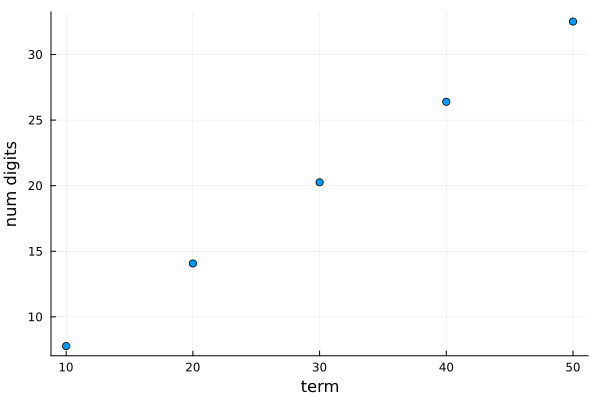
absErr(4*(atan_series(1/2,20)+atan_series(1/3,20)))

🔗

which is 7.993605777301127e-15, so about 14 digits. You should notice that quite quickly, the value is converging. Since we are quickly running out of precision for 64-bit floats, we will switch to BigFloats and quite easily with:

🔗

 4*(atan_series(1/big(2),20)+atan_series(1/big(3),20))

🔗

which returns

🔗

3.141592653589801775394859982612606961085892242193168775435423632752985359741545

🔗

Let’s visually see how quickly this is converging. First, we’ll find the errors with:

🔗

 errors2=map(n -> absErr(4*(atan_series(1/big(2), 10n) + atan_series(1/big(3), 10n))), 1:5)

🔗

which returns

🔗

5-element Vector{BigFloat}:
  1.686089269049955549324338738573041181676956757596130409476023763757476121934317e-08
  8.536932216599333104076888722842818062954460479040445168953455346681077569196179e-15
  5.541360098004753291440085860743946761847969162268014510791810751138256936210001e-21
  4.005347048909364704518520476811412326265959273017889120734252574465535050431139e-27
  3.075296346725383632749782433311833539450331895967037047902902585859740513243069e-33

🔗

 scatter(10:10:50, -log10.(errors2), legend=false)

🔗

which results in

🔗

The slope of this line is about \(0.6\text{,}\) which implies that every 10 terms results in another 6 digits of accuracy. Using the plot, we estimate that 100 digits would give an accuracy of over 60 digits and

🔗

 @time absErr(4*(atan_series(1/big(2),100)+atan_series(1/big(3),100)))

🔗

took 0.000251 seconds and has a accuracy of about 63 digits.

🔗

which 5 times as many digits and is much faster than the estimated 245,000 years that the previous method was predicted to take.

🔗

Since the default number of decimal digits for a BigFloat is about 78 decimal places, we again will quickly run out of precision. Let’s try to see about finding \(\pi\) to 1000 digits. We’re going to adjust the precision of BigFloats, but instead of setting in everywhere we can set it on a block of code with

🔗

setprecision(4096) do 
# run code here 
end

🔗

then the number of digits of precision can be seen with

🔗

setprecision(4096) do 
  length(string(1/big(3))) 
end

🔗

which creates the BigFloat 1/3, turns it to a string and finds the length. The result is 1237, so this is plenty to calculate to 1000 digits.

🔗

To estimate the number of terms needed for 1000 digits, a line fitting the data above is about \(d=-0.625(n-20)-14\text{.}\) So a little algebra for letting \(d=-1000\text{,}\) results in \(20-984/-0.625= 1594\) terms. Entering:

🔗

setprecision(4096) do 
  @show pi1000=4*(atan_series(1/big(2),1594)+atan_series(1/big(3),1594)) 
  absErr(pi1000)
end

🔗

results in

🔗

pi1000 = 4 * (atan_series(1 / big(2), 1594) + atan_series(1 / big(3), 1594)) = 3.1415926535897932384626433832795028841971693993751058209749445923078164062862089986280348253421170679821480865132823066470938446095505822317253594081284811174502841027019385211055596446229489549303819644288109756659334461284756482337867831652712019091456485669234603486104543266482133936072602491412737245870066063155881748815209209628292540917153643678925903600113305305488204665213841469519415116094330572703657595919530921861173819326117931051185480744623799627495673518857527248912279381830119491298336733624406566430860213949463952247371907021798609437027705392171762931767523846748184676694051320005681271452635608277857713427577896091736371787214684409012249534301465495853710507922796892589235420199561121290219608640344181598136297747713099605187072113499999983729780499510597317328160963185950244594553469083026425223082533446850352619311881710100031378387528865875332083814206171776691473035982534904287554687311595628638823537875937519577818577805321714865601239565154256531508207949971669743165722740018351762297978126407660203701569790495607661311942951883071049126683863914353996276446515815532113161156858922687498386163189387937947070163492538574522358773840865866641344202158314334039229961783600168318495477941285685
 2.5975351095458754904195491157857696803622131507293634931295093187648738419240192667709752546427822529941468450549877713666966011614851313600669596886196498994143921672175459108290471960863459461639251291662232368565896246328120598260939106463457479630917174483761218561210120412869465176525005824807899438481196329993790493359900522454759482318202266105921331249007978097775724687956301642633550860637174924190228399842631614879639158046917042635291042631965291845166527036203452319813178296082929894900734880740547269432828997961816403444163166354514484699977363284177623290122184020750178932873624933570074682872942723076449879540864947698524422632479056630893008599428469562364494768790325744031011930601596329086026289242110179341279393200929314660273031057473081913078692798691499162555114494444741975803032974623739919031238086655685280832758980871795419698822680825529239750189369473347847251964195124706746244861133322038379060583915976636069455518781609572437864178386621806568957217481465862297442152542221932061173187093506126070914995792754149603406706779637343994385988667569337732890340690567393340395500287349361658707200982844137221365907346244068359959729947248038871713897283543740693133197921478035649291888640453449e-964

🔗

The exponential terms is 10 to the \(-964\text{,}\) that is about 964 digits of accuracy. Obviously this didn’t find \(\pi\) to the required 1000 digits. Our estimate was off a bit. Before we adjust this, note that we are really just interested in the number of digits, we can find by taking the log of the result or more-specifically:

🔗

numDigits(pi_approx::Real) = floor(Int,-log10(absErr(pi_approx)))

🔗

So instead, let’s

🔗

setprecision(4096) do 
  pi1000=4*(atan_series(1/big(2),1594)+atan_series(1/big(3),1594)) 
  numDigits(pi1000)
end

🔗

which will return 963.

🔗

Since the 1594 was an estimate, let’s bump up the number of terms to 1700:

🔗

@time setprecision(4096) do
  pi1000=4*(atan_series(1/big(2),1700)+atan_series(1/big(3),1700))
  numDigits(pi1000)
end

🔗

which showed the number of digits is 1027 and took 0.072266 seconds.

🔗

Section 48.3 Speed of the arctangent series

Much of this chapter is about speed. We want to be able to calculate \(\pi\) in a reasonable amount of time. We can actually speed up the algorithm in a way similar to the Horner’s form as in Subsection 28.2.1 in the following way. If we write (48.2) in the following way:

🔗

\begin{equation*} \tan^{-1} = x \biggl(1-x^2\biggl(\frac{1}{3}-x^2 \biggl(\frac{1}{5} -x^2 \biggl(\frac{1}{7} -x^2\biggl(\cdots \biggr)\biggr)\biggr)\biggr)\biggr) \end{equation*}

🔗

we can sum this faster. Consider

🔗

function atan_series2(x::Real,n::Integer)
  n > 0 || throw(ArgumentError("The input n must be positive."))
  local negxsq = -x^2
  local sum = 1.0
  local ak = 1.0
  for k=2:n
    ak *= negxsq
    sum += ak/(2k-1)
  end
  x*sum
end

Some of the ways this speeds up is by first calculating \(-x^2\) and this is the only power of \(x\) calculated. Then sums of this term are made. To test the speed, let’s first use the BenchmarkTools package and repeat the example above:

🔗

@btime setprecision(2^14) do 
  numDigits(4*(atan_series(1/big(2),1700)+atan_series(1/big(3),1700))) 
end

🔗

which results in 395.834 msand using the new series with

🔗

@btime setprecision(2^14) do 
  numDigits(4*(atan_series2(1/big(2),1700)+atan_series2(1/big(3),1700))) 
end

🔗

and this results in 39.631 ms which is a 10 times speed enhancement.

🔗

Section 48.4 If I had a million dollars digits

With apologies to the Barenaked Ladies,

The Barenaked Ladies is a Canadian rock band, which the author was a fan of. One of their biggest hits was If I had a Million Dollars.

let’s see how feasible it is to find \(\pi\) to a million digits. First, we need to make sure that we use a large enough BigFloat. If we try

🔗

setprecision(2^14) do
  length(string(1/big(3))) 
end

🔗

using \(2^{14}\) or 16384 bits results in a BigFloat with 4936 decimal digits. If you play with the power on the precision, note that we need a minimum of \(2^{22}\) binary digits, this should be enough. However, note that at this level of precision, calculations slow down quite a bit. For example,

🔗

@time setprecision(2^22) do 
  numDigits(4*(atan_series2(1/big(2),100)+atan_series2(1/big(3),100))) 
end

🔗

shows that the same 63 digits of accuracy took 13.153726 seconds. Also, it can be checked that doubling the number of terms will double the number of digits as well as doubling the time. It’s estimated it would take 58 hours to use this method to find \(\pi\) to 1 million digits.

🔗

Section 48.5 Machin’s Formula and related Formulas

The reason that Euler’s formula worked much better that the first method is that it calculated the arctangents of \(1/2\) and \(1/3\text{.}\) This converges relatively quickly in that power series are powers of \(1/2\) and \(1/3\text{.}\) If we can develop similar formula for fractions closer to zero, this may converge even faster.

🔗

Machin in 1706 noticed the relationship

🔗

\begin{equation} \frac{\pi}{4} = 4 \tan^{-1} \frac{1}{5} - \tan^{-1} \frac{1}{239}\tag{48.4} \end{equation}

🔗

and was able to extend what Euler did as well in a much more efficient manner as we will see below. There are a lot of known Machin-type formula that exist (and check out Wikipedia site for some examples). In the 1970s and 1980s with the accelerated power of computers, many mathematicians and computer scientists founds many other formulas like (48.4). For example, in 1982, Kikuo Takano showed that

🔗

\begin{align} \frac {\pi }{4} = \amp 12\arctan\biggl(\frac {1}{49}\biggr)+32\arctan\biggl(\frac {1}{57}\biggr)\notag\\ \amp \qquad -5\arctan\biggl(\frac {1}{239}\biggr)+12\arctan\biggl(\frac {1}{110443}\biggr). \tag{48.5} \end{align}

🔗

And for \(\pi\)-day in 2024, Matt Parker

A favorite of the author who has both a podcast and youtube channel with fascinating and entertiaining mathematical-related material.

covened many people to hand calculate \(\pi\text{.}\) This group used the following relationship:

🔗

\begin{align} \frac{\pi}{4} = \amp 83 \tan^{-1} \frac{1}{107}+ 17 \tan^{-1} \frac{1}{1710} -22 \tan^{-1} \frac{1}{103697} \notag\\ \amp \qquad -24 \tan^{-1} \frac{1}{2513489} -44 \tan^{-1} \frac{1}{18280007883} \notag\\ \amp \qquad +12 \tan^{-1} \frac{1}{7939642926390344818} \notag\\ \amp \qquad + 22 \tan^{-1} \frac{1}{3054211727257704725384731479018} \tag{48.6} \end{align}

🔗

Subsection 48.5.1 Using Machin’s Formulas to Calculate \(\pi\)

Notice that in (48.3), (48.4), (48.5) and (48.6), they are all linear combinations of integer coefficients with arctangents of 1 over an integer. Because of this, we can write the following Julia function to calculate all of these:

🔗

function machin(coeffs::Vector{Int}, xvals::Vector{T},n::Int) where T <: Integer
  length(coeffs) == length(xvals) || throw(ArgumentError("The lengths of the vectors must match"))
  local sum=big(0)
  for i=1:length(coeffs)
    sum += coeffs[i]*atan_series2(1/big(xvals[i]),n)
  end
  4*sum
end

Then for a testing example, we can reproduce the Euler formula with

🔗

setprecision(2^14) do 
  numDigits(machin([1,1],[2,3],100)) 
end

🔗

and this returns 62. Use this on Machine’s formula in (48.4) and we’ll put the precision back to handling a million digits and the following

🔗

@time setprecision(2^22) do 
  numDigits(machin([4,-1],[5,239], 100)) 
end

🔗

results in 141 digits of accuracy in 11.025900 seconds. If we double the number of terms used from 100 to 200, the time roughly doubles to 19.208941 seconds. and the number of terms goes to 352. This would seem to show that to get to million digits would take just about 19 hours, which is shorter than Euler’s method, but not great.

🔗

If we apply the Takano’s formula in (48.5) with

🔗

@time setprecision(2^22) do 
  numDigits(machin([44,7,-12,24],[57,239,682,12943], 100)) 
end

🔗

this shows that we get 352 digits of accuracy in 16.688353 seconds. Again, doubling the number of terms doubles both the accuracy (704 digits) and the time it takes (27.553502 seconds). Again, extrapolating, Takano’s method would take 10.87 hours to do 1 million digits.

🔗

And lastly, the formla that Matt Parker used in (48.6) can be calculated with

🔗

@time setprecision(2^22) do
  numDigits(machin([83,17,-22,-24,-44,12,22],
    [big(107),big(1710),big(103697),big(2513489),big(18280007883),big(7939642926390344818), big(3054211727257704725384731479018)], 100))
end

🔗

which resulted in 407 digits of accuracy in 25.319640 seconds. Again, doubling the number of terms used doubled the accuracy to 813 digits and took 43.706857 seconds. Extrapolating this would result in a million digits in 14.93 hours. Notice that each of these Machin’s formulas are good, but would take quite a bit of computing time. Notice that the method of Parker was slower than Takano’s formula, but the goal of Matt Parker was to calculate this by hand using the formula.

For a bit of a spoiler, the group calculated \(\pi\) to 120 digits during a week of work.

🔗

Section 48.6 The Chudnovsky Brothers and Ramanujan

There is a fascinating article in the March 2, 1992 issue of the New Yorker magazine (provide ref) A pair of brothers with last name Chudnovsky built a supercomputer out of mail-order parts in their New York City apartment with the goal of finding the digits of \(\pi\text{.}\) They used the following series:

🔗

\begin{equation} \frac{1}{\pi} = 12 \sum_{k=0}^{\infty} \frac{ (-1)^k (6k)! (545140134 k + 13591409)}{(3k)! (k!)^3 (640320^3)^{k+1/2}}\tag{48.7} \end{equation}

🔗

which was originally attributed to Ramanujan.

⁴

I won’t get into the details of the story here or Ramanujan, but the New Yorker story is a easy and great read and learning about Ramanujan is yet another wonderful tangent.

🔗

This equation can be written as

🔗

\begin{align} \frac{1}{\pi} \amp = \frac{12}{\sqrt{640320^3}} \sum_{k=0}^{\infty} a_k (545140134 k + 13591409)\tag{48.8}\\ \amp = \frac{12}{\sqrt{640320^3}} \biggl( 545140134 \sum_{k=0}^{\infty} k a_k + 13591409 \sum_{k=0}^{\infty} a_k \biggr) \tag{48.9}\\ \amp \qquad \qquad \text{where}\notag\\ a_k \amp = \frac{ (-1)^k (6k)!}{(3k)! (k!)^3 640320^{3k}}\notag \end{align}

🔗

If we let

🔗

\begin{equation*} S = \biggl( 545140134 \sum_{k=0}^{\infty} k a_k + 13591409 \sum_{k=0}^{\infty} a_k \biggr) \end{equation*}

🔗

then using (48.9) we can solve for \(\pi\) with:

🔗

\begin{equation} \pi = \frac{\sqrt{640320^3}}{12S}\tag{48.10} \end{equation}

🔗

We can do this in julia with the following:

🔗

function chud(n::Integer)
  sum = big(0)
  for k=0:n
    ak =  (-1)^k*factorial(big(6k))/factorial(big(3k))/ factorial(big(k))^3/ (big(640320)^3)^(k+0.5)
    sum += big(545140134)*k*ak + big(13591409)*ak
  end
  1/(12sum)
end

and let’s check out it’s performance by a comparison to Takano’s method above:

🔗

@time setprecision(2^22) do 
  numDigits(chud(20)) 
end

🔗

and the result shows that this calculates \(\pi\) to 297 digits and took 145 seconds. Note that we only used 20 terms for this calculation. Before, trying to determine the total time to get to 1 million digits, we can use some of the same techniques that we used to speed up the arctangent series in the function atan_series2 as

🔗

function chudnovsky(n::Integer)
  local sum1 = big(1.0)
  local sum2 = big(0.0)
  local top = big(1)
  local bottom = big(1)
  local C = big(640320)^3
  for k=1:n
    top *= -24*(6*k-5)*(2*k-1)*(6*k-1)
    bottom *= C*k^3
    sum1 += top/bottom
    sum2 += k * top/bottom
  end
  426880*sqrt(big(10005))/(13591409*sum1 + 545140134*sum2)
end

and computing the first 20 terms of this using:

🔗

@time setprecision(2^22) do 
  numDigits(chudnovsky(20)) 
end

🔗

results in the same 297 terms (which is good that we got the same results) in 7.862153 seconds.

🔗

and try with twice as many terms with:

🔗

@time setprecision(2^22) do 
  numDigits(chudnovsky(40)) 
end

🔗

and the result is 581 digits in 10.962281 seconds and if we go to 80 terms, then we get 1148 terms in 15.179335 seconds. The relationship seems to be roughly linear, so we expect the total time to calculate \(\pi\) to a million digits would be about 3.67 hours.

🔗

Subsection 48.6.1 A parallel version of the Chudnovsky Algorithm

All of the algorithms here in this chapter can be adapted for parallelization because the sums can be split into pieces to be distributed over multiple processors or cores. If you need to, you may want to review the material in Chapter 29 for background on distributed computing in julia.

🔗

 using Distributed

🔗

We rewrite the chudnovsky function so it can be parallelized. We want to be able to break up the sum in (48.8) to sum between \(n_1\) and \(n_2\text{.}\)

🔗

@everywhere function paraChud(n1::Integer,n2::Integer,prec::Integer)
  setprecision(prec)
  local C = big(640320)^3
  local bottom = big(1)
  local top = big(1)
  for k=1:n1
    bottom *= k^3*C
    top *= -8*(6k-1)*(6k-3)*(6k-5)
  end
  local sum1 = n1*top/bottom
  local sum2 = top/bottom
  for k=n1+1:n2
    bottom *= k^3*C
    top *= -8*(6k-1)*(6k-3)*(6k-5)
    sum1 += k*top/bottom
    sum2 += top/bottom
  end
  545140134*sum1 + 13591409*sum2
end

A number of comments about this function:

🔗

On line 1, recall that @everywhere is needed for parallelization.
🔗

🔗
Also due to parallelization, we need to set the precision on each core/processor, so the precision is passed into the function and set on line 2.
🔗

🔗
Line 3--11, build up the values of bottom and top needed for the 2nd for loop. These are needed because instead of actually calculating the factorial, we build up the values term by term. Note, we also keep the terms bottom and top as BigInts for speed instead of calculating each term as a BigFloat.
🔗

🔗
The for loop in lines 12--17 repeat the calculations for the terms, however in this case calculate the terms for sum1 and sum2.
🔗

🔗
The number that is returned is the number in (48.8) in the parentheses for the terms \(n_1\) through \(n_2\text{.}\) This doesn’t return \(\pi\) because we need to add the terms up first.
🔗

🔗

🔗

An example of how to use this function (although not in a parallel fashion) is

🔗

@time let
  prec = 2^22
  p1 = paraChud(0,9,prec)
  p2 = paraChud(10,19,prec)
  p3 = paraChud(20,29,prec)
  p4 = paraChud(30,39,prec)
  numDigits(sqrt(big(640320)^3)/(12*(p1+p2+p3+p4)))
end

🔗

which returns:

🔗

Note that p1 through p4 calculate 10 terms of the series each. Then the last line is the equation (48.10) and for \(\pi\text{.}\)

🔗

To do parallelization, we can adapt from above using the pmap function, which recall, does parallel map. We can repeat the above line as:

🔗

@time setprecision(2^22) do 
  local p = pmap(i -> paraChud(10*(i-1),10i-1,2^22),1:4) 
  local s = sum(p) 
  numDigits(sqrt(big(640320)^3)/(12s)) 
end

🔗

which returns nearly the same number of digits (597) in 8.644556 seconds just a bit smaller than the non parallel version. The machine that I am using has 8 cores, so we’ll change the end of the second line to 1:8 or

🔗

@time setprecision(2^22) do 
  local p = pmap(i -> paraChud(10*(i-1), 10i-1, 2^22),1:8) 
  local s = sum(p) 
  numDigits(sqrt(big(640320)^3)/(12s)) 
end

🔗

which will double to the number of digits to 1134 in 11.959962 seconds.

🔗

Cranking up to a total of 800 terms with

🔗

@time setprecision(2^22) do 
  local p = pmap(i->paraChud(100*(i-1),100i-1,2^22),1:8) 
  local s = sum(p) 
  numDigits(sqrt(big(640320)^3)/(12s)) 
end

🔗

resulted in 11345 digits of accuracy in 48.279909 seconds and using this method would be predicted that we could calculate \(\pi\) to just over 1 million digits in about 71 minutes. This was on my 8-core Macbook Air. Just for comparison, the New Yorker article cited above mentioned that the Chudnovsky brothers computed \(\pi\) to more that 1 billion digits. It didn’t mention how long it took.

🔗

You can’t just take the 18 minutes and multiply by 1000 to get to a billion digits because I used the floating-point precision that was just over a million and would have to scale that.

🔗

Check Your Understanding 48.3.

(a)

Parallelize the machin and atan_series2 functions above. Note: you will need to do similar techniques to that in the paraChud function.

🔗

(b)

Test these by comparing to the non parallelized versions.

🔗

Prev Top Next