Differential Equations

Chapter 43 Differential Equations

Another extremely important topic in Scientific Computation is that of differential equations. These arise obviously in mathematics, but also in most other scientific fields including biology, chemistry, engineering, and economics. Also, it is rare that a differential equation has a nice closed form solution, so often numerical methods must be used to get a solution.

🔗

We will discuss two often-used methods for solving differential equations, Euler’s method and Runge-Kutta methods and then delve into a very nice robust julia package.

🔗

A differential equation is simply an equation that has derivatively in it. For example

🔗

\begin{equation*} y'' + 4 y = 0 \end{equation*}

🔗

It is important to note that the order of a differential equation is the degree of the highest derivative, so in the example above, it is two. The following procedure can covert non order-1 differential equation to one that is a first-order system.

🔗

Let \(y_1 = y\text{,}\) then \(y_2 = y' = y_1'\text{.}\) Lastly \(y'' = y_1'' = y_2'\) and using the differential equation \(y''=-4y\text{,}\) this can be written:

🔗

\begin{align*} y_1' \amp = y_2 \\ y_2' \amp = -4y_1 \end{align*}

🔗

or in matrix form:

🔗

\begin{equation*} \begin{bmatrix} y_1 \\ y_2 \end{bmatrix}' = \begin{bmatrix} y_2 \\ -4y_1 \end{bmatrix} \end{equation*}

🔗

and as long as \(y^{(n)}\text{,}\) the highest-order term, can be isolated algebraically, one can write the differential equation as

🔗

\begin{equation*} \mathbf{y}' = F(\mathbf{y}) \end{equation*}

🔗

Section 43.1 Euler’s Method

We start with one of the simplest methods to solve a differential equation. If we have are solving

🔗

\begin{equation} y' = f(y,t), \qquad y(0) = y_0\tag{43.1} \end{equation}

🔗

with the understanding that we will solve this at a discrete set of points, so we let \(y_n = y(t_n)\) and \(t_k = t_0 + k\Delta t\text{,}\) where \(\Delta t\) is a small time step. We can then replace \(y'\) with the approximation:

🔗

\begin{equation*} y' \approx \frac{y_{n+1}-y_n}{t_{n_1}-t_n} \end{equation*}

🔗

and the differential equation in (43.1) is

🔗

\begin{equation*} \frac{y_{n+1}-y_n}{t_{n_1}-t_n} = \frac{y_{n+1}-y_n}{\Delta t} = f(y_n,t_n) \end{equation*}

🔗

and solving for \(y_{n+1}\text{,}\) we get:

🔗

\begin{equation*} y_{n+1} = y_n + \Delta t f(y_n,t_n) \end{equation*}

🔗

and this iterative (or difference equation) is known as Euler’s Method.

🔗

Subsection 43.1.1 Implementing Euler’s method in Julia

Let’s take a look at Euler’s method in Julia. Of course, we’ll write a function to evaluate this and there are a few things that we need for the function:

🔗

The function \(f\text{,}\) which is the right-hand side. Note that it takes in two variables.
🔗

🔗
An initial point, \((t_0,y_0)\text{.}\) There will be two real arguments for this.
🔗

🔗
A step size \(\Delta t\text{.}\)
🔗

🔗
Either a final \(t\) value or a number of steps to run Euler’s method. We’ll use the number of steps, a positive integer.
🔗

🔗

🔗

We’ll return two arrays for the t and y values.

🔗

We’ll also implement this as a for loop. Although there are some

🔗

function euler(f::Function, t0:: Real, y0::Real, dt::Real, num_steps::Integer)
  num_steps > 0 || throw(ArgumentError("The number of steps must be positive."))
  dt > 0 || throw(ArgumentError("The step size dt must be positive."))
  t = LinRange(t0,t0+num_steps*dt,num_steps+1)
  y = zeros(Float64,num_steps+1)
  y[1] = y0
  for i=1:num_steps
    y[i+1] = y[i] + dt*f(t[i],y[i])
  end
  (t,y)
end

Example 43.1.

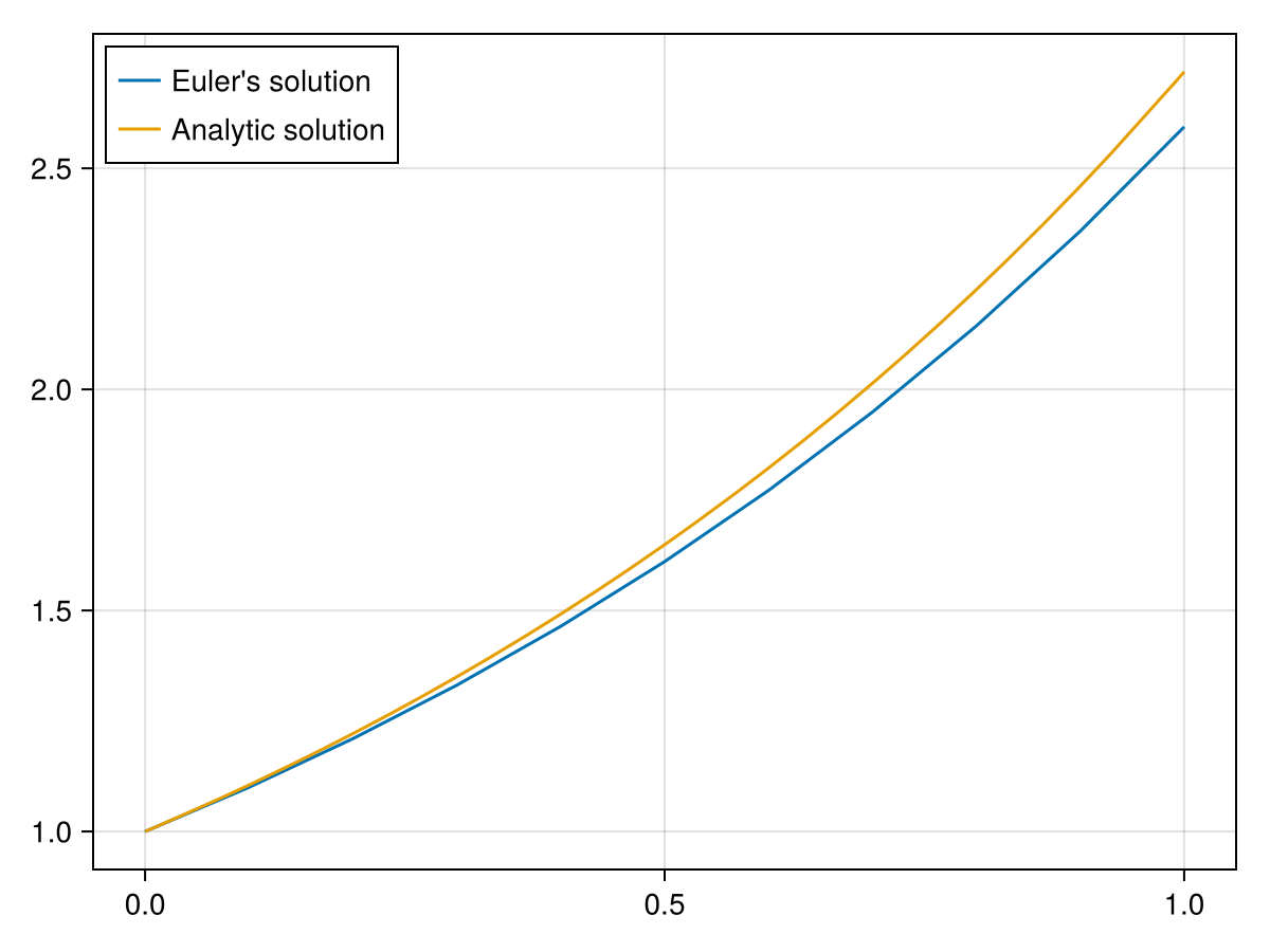
We’ll solve \(y'=y\text{,}\) \(y(0)=1\) for dt=0.1 and \(10\) steps.

t,y = euler( (t,y) -> y, 0, 1, 0.1, 10)

🔗

and this returns

🔗

([0.0, 0.1, 0.2, 0.3, 0.4, 0.5, 0.6, 0.7, 0.8, 0.9, 1.0], [1.0, 1.1, 1.2100000000000002, 1.3310000000000002, 1.4641000000000002, 1.61051, 1.7715610000000002, 1.9487171, 2.1435888100000002, 2.357947691, 2.5937424601])

🔗

which is a tuple of two arrays. This results the \(t\) and \(y\) values based on Euler’s method. However, perhaps it’s more interesting to see a plot. Also, note that the analytic solution to this is \(y=e^x\text{,}\) so the plot of the approximate solution using Euler’s method as well as the analytic solution is

🔗

fig, ax = lines(t,y,label="Euler's solution")
lines!(ax, 0..1, exp,label="Analytic solution")
axislegend(ax, position = :lt)
fig

🔗

🔗

Section 43.2 Runge Kutta methods

There is a family of other methods called the Runge Kutta methods that are relatively simple with a high order of accuracy. One version that was often a standard version is what is called the 4th-order Runge-Kutta or RK4 method is

🔗

\begin{equation*} y_{n+1} = y_n + \frac{h}{6} \bigl(k_1+2k_2+2k_3+k_4 \bigr) \end{equation*}

🔗

where

🔗

\begin{align*} k_1 \amp = f(t_n,y_n) \\ k_2 \amp = f\biggl(t_n + \frac{h}{2}, y_n + \frac{h}{2} k_1 \biggr) \\ k_3 \amp = f\biggl(t_n + \frac{h}{2}, y_n + \frac{h}{2} k_2 \biggr) \\ k_4 \amp = f(t_n + h, y_n + h k_3 \biggr) \end{align*}

🔗

Subsection 43.2.1 RK4 in julia

The following is the rk4 method in julia. It is very similar to euler’s method...

🔗

function rk4(f::Function, t0:: Real, y0::Real, dt::Real, num_steps::Integer)
  num_steps > 0 || throw(ArgumentError("The number of steps must be positive."))
  dt > 0 || throw(ArgumentError("The step size dt must be positive."))
  t=LinRange(t0,t0+num_steps*dt,num_steps+1)
  y=zeros(Float64,num_steps+1)
  y[1] = y0
  for i=1:num_steps
    k1 = f(t[i],y[i])
    k2 = f(t[i]+dt/2,y[i]+dt/2*k1)
    k3 = f(t[i]+dt/2,y[i]+dt/2*k2)
    k4 = f(t[i]+dt,y[i]+dt*k3)
    y[i+1] = y[i] + dt/6*(k1+2k2+2k3+k4)
  end
  (t,y)
end

and we can use this to solve \(y'=y\text{,}\) \(y(0)=1\) by

🔗

t,y = rk4((t,y) -> y, 0, 1, 0.1, 10)

🔗

and the results are

🔗

(LinRange{Float64}(0.0, 1.0, 11), [1.0, 1.1051708333333332, 1.2214025708506944, 1.3498584970625376, 1.4918242400806856, 1.648720638596838, 1.822117962091933, 2.0137516265967768, 2.2255395632923154, 2.459601413780071, 2.718279744135166])

🔗

Section 43.3 Using the `DifferentialEquations package`

There is a very mature and robust package for solving differential equations aptly called DifferentialEquations. We will show a few examples to get a feeling for how to use the package, but as you can tell from the documentation, that there are a lot of possibilities with the package so we’ll show a couple of examples.

🔗

In short, you’ll need to include the equation, an initial condition and a range of values on which you want it solved. Don’t forget to add the package and evaluate

🔗

using DifferentialEquations

🔗

Subsection 43.3.1 A Simple Example

We will solve

🔗

\begin{equation*} \frac{dy}{dt} = y \qquad y(0)=1 \end{equation*}

🔗

the same equation as above using the DifferentialEquations package.

🔗

First, the equation needs to fit in the form:

🔗

\begin{equation*} \frac{du}{dt} = f(u,p,t) \end{equation*}

🔗

where \(f\) is a function of \(u\text{,}\) the dependent variable, \(p\) the parameter in the problem (if any) and \(t\text{,}\) the independent variable. We will also defined the initial condition and the range of values for which to solve:

🔗

f(u,p,t) = u
u0 = 1.0
tspan = (0.0,1.0)

🔗

And then we create a differential equation problem with:

prob = ODEProblem(f,u0,tspan)

🔗

and note that this returns

🔗

ODEProblem with uType Float64 and tType Float64. In-place: false
timespan: (0.0, 1.0)
u0: 1.0

🔗

This gives information about the datatypes of the function and initial condition because some solvers will use this information differently. to solve this problem,

🔗

 sol = solve(prob)

🔗

which returns

🔗

retcode: Success
Interpolation: 3rd order Hermite
t: 5-element Vector{Float64}:
 0.0
 0.10001999200479662
 0.34802032833535873
 0.683052570376323
 1.0
u: 5-element Vector{Float64}:
 1.0
 1.105193012902056
 1.416261037790314
 1.9799122839671017
 2.718281708773355

🔗

Note that the solution appears to be an array of time (that isn’t equally-spaced) and function values at those \(t\) values. If you want to access one of them, you can do:

🔗

 sol[3]

🔗

which returns 1.416261037790314, the third element of the u array. However, this structure is much more than just an array. If you want the function value at 0.75, for example, you can access it like a function evaluation:

🔗

 sol(0.75)

🔗

which returns 2.1170003461681204 and this is interpolated from the generated points. The result guarantees accuracy to within a default tolerance of 1e-3 or you can set a different tolerance with the keyword reltol such as reltol=1e-6.

🔗

So for example, you can generate an array of tuples with

🔗

[(t,sol(t)) for t=0:0.1:1]

🔗

which returns

🔗

11-element Vector{Tuple{Float64, Float64}}:
 (0.0, 1.0)
 (0.1, 1.1051709180988993)
 (0.2, 1.2214028012281672)
 (0.3, 1.3498587272674625)
 (0.4, 1.4918249699503803)
 (0.5, 1.648721181273569)
 (0.6, 1.8221180994290354)
 (0.7, 2.0137527117177667)
 (0.8, 2.2255411035915857)
 (0.9, 2.4596023119414028)
 (1.0, 2.718281708773351)

🔗

One can also generate a plot of the solution with

lines(pts)

🔗

or if you want to plot the numerical solution with the analytic solution \(y=e^t\text{,}\) then

🔗

fig, ax = lines(pts)
lines!(0..1,exp)
fig

🔗

and the result is

🔗

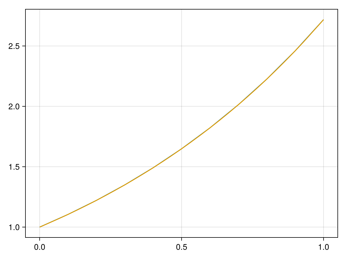
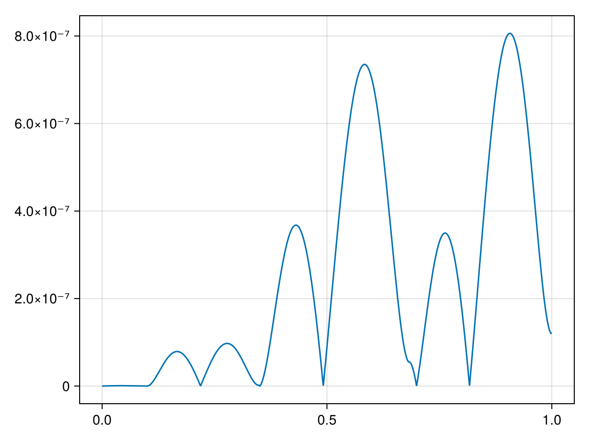
which shows that they appear to the resolution of the plot that the two solutions are identical, however if we plot the error associated with the numerical method by

🔗

lines(0..1, t -> abs(sol(t)-exp(t)))

🔗

which generates the following plot:

🔗

this shows that error is within \(10^{-6}\text{,}\) which is the tolerance for the solve method of the DifferentialEquations package.

🔗

Check Your Understanding 43.5.

(a)

Find the solution to the differential equation

🔗

\begin{equation*} y' = \frac{t}{1+y^2}, \qquad y(0) = 1 \end{equation*}

🔗

on the interval \([0,10]\text{.}\)

🔗

(b)

Reproduce the solution to \(y'=y, ~~ y(0)=1\) with the option abstol = 1e-10. Produce a plot of the error as above to show that the result is within the given tolerance.

🔗

Section 43.4 Example of a system of differential equations

Let’s solve

🔗

\begin{equation*} y'' + y = 0 \end{equation*}

🔗

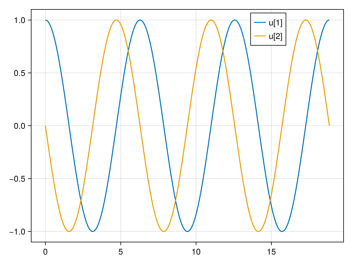
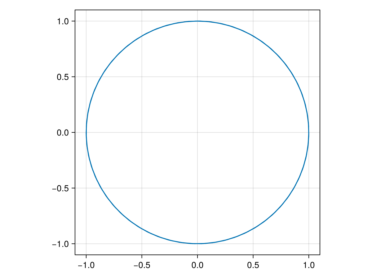
which is an example of a harmonic oscillator. We first need to put this in a system form by letting \(y_1=y\) and \(y_2=y'\text{.}\) Then from the differential equation \(y'' = - y\) or \(y_2' = -y_1\text{.}\) We can then write this as

🔗

\begin{align*} y_1' \amp = y_2 \\ y_2' \amp = -y_1 \end{align*}

🔗

We will write this in julia using

🔗

function F!(du,u,p,t) 
  du[1] = u[2] 
  du[2] = - u[1] 
end

🔗

and then create the differential problem with

🔗

 prob2 = ODEProblem(F!,[1;0],(0,6pi))

🔗

where [1;0] is the initial condition which would be \(y(0)=1, y'(0)=0\) and the solution is

🔗

 sol2 = solve(prob2)

🔗

If you just plot the results:

🔗

fig, ax = lines(sol3)
axislegend(ax, position=(0.8,1))
fig

🔗

you’ll see the two elements of the vector plotted as functions of \(t\) or:

🔗

If instead, you want the results plotted like a parametric equation, then we need to do a bit more work. The result of the solution sol2 is a function of t that returns a vector of the two variables \(y_1\) and \(y_2\text{.}\) To generate the desired plot:

🔗

y1 = map(t -> sol3(t)[1],0:0.1:6pi)
y2 = map(t -> sol3(t)[2],0:0.1:6pi)
lines(y1, y2, axis = (aspect = 1,))

🔗

and recall that the comma afer aspect = 1, is important to make that a tuple and we desire the aspect ratio to be 1 because the output should be a circle. The plot is

🔗

Subsection 43.4.1 The Lorenz System

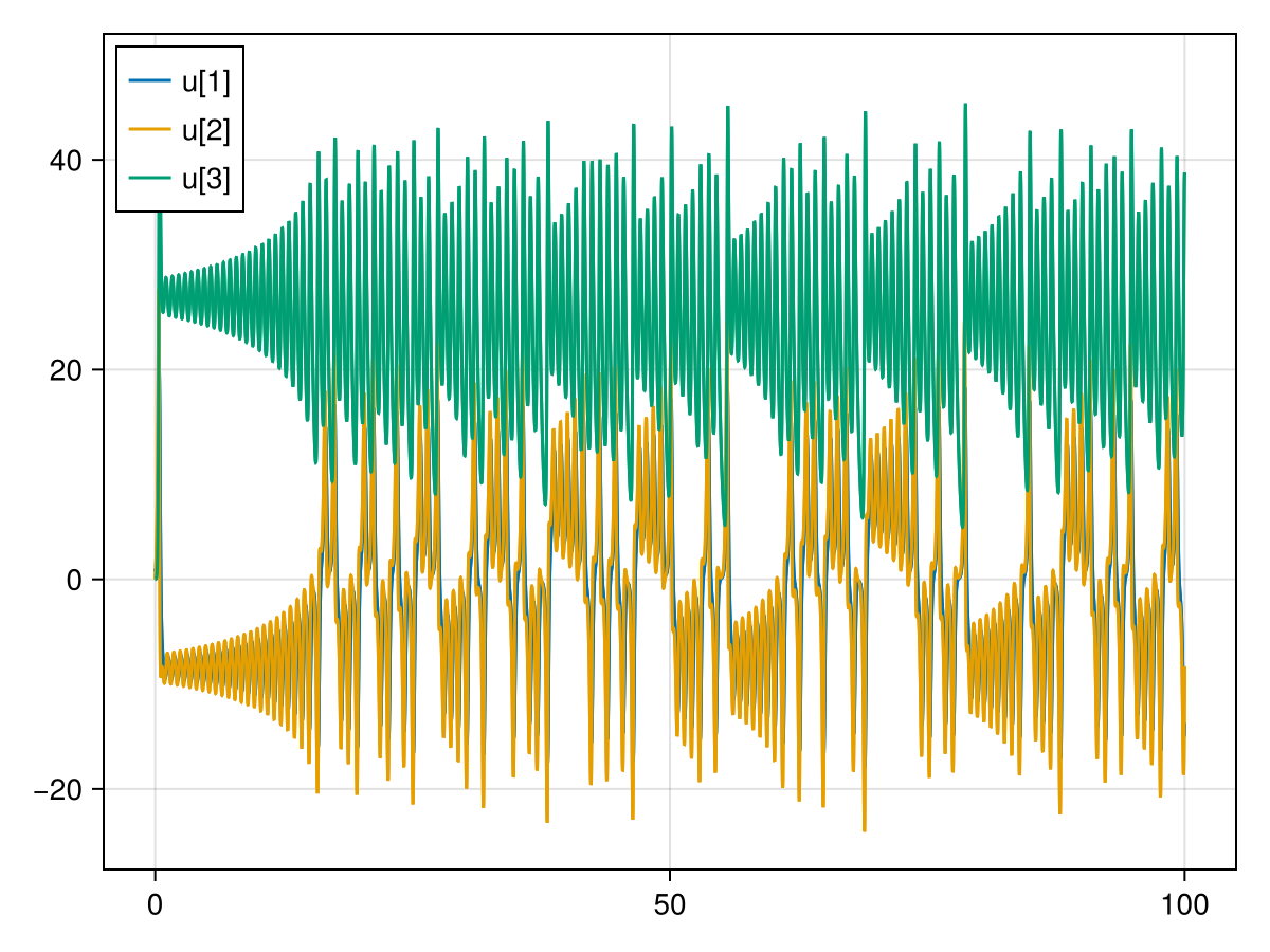
The Lorenz system is relatively famous system of differential equations for many reasons. It is a system of ODEs, it is nonlinear and for many parameters the solution exhibits sensitivity on initial conditions, an important property for differential equation that exhibit chaotic behavior. The Lorenz system is

🔗

\begin{align*} \frac{dx}{dt} \amp = \sigma (y-x) \\ \frac{dy}{dt} \amp = x (\rho -z) - y \\ \frac{dz}{dt} \amp = xy - \beta z \end{align*}

🔗

and we will look for solution with \(\sigma=10, \rho = 28\) and \(\beta=8/3\) so we define

🔗

function lorenz!(du, u, p, t)
  du[1] = 10.0 * (u[2] - u[1])
  du[2] = u[1] * (28.0 - u[3]) - u[2]
  du[3] = u[1] * u[2] - (8 / 3) * u[3]
  nothing
end

🔗

and if the following timespan and initial conditions are used to solve the differential equation as in:

🔗

u0 = [1.0; 0.0; 0.0]
tspan = (0.0, 100.0)
prob = ODEProblem(lorenz!, u0, tspan)
solve(prob);

🔗

If we plot the 3 components of the solution as functions of t, with

🔗

fig, ax = lines(lorsol)
axislegend(ax, position = :lt)
fig

🔗

and the plot is

🔗

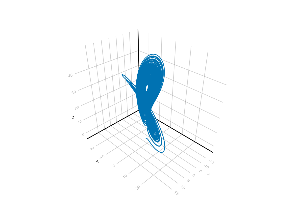
and it is difficult to see the difference between u[1] and u[2]. The classic plot of this solution is as a 3D parametric plot, which can be generated with

🔗

t = LinRange(0,100,10_000)
lines(lorsol(t,idxs = 1).u, lorsol(t, idxs = 2).u, lorsol(t, idxs = 3).u)

🔗

and this results in

🔗

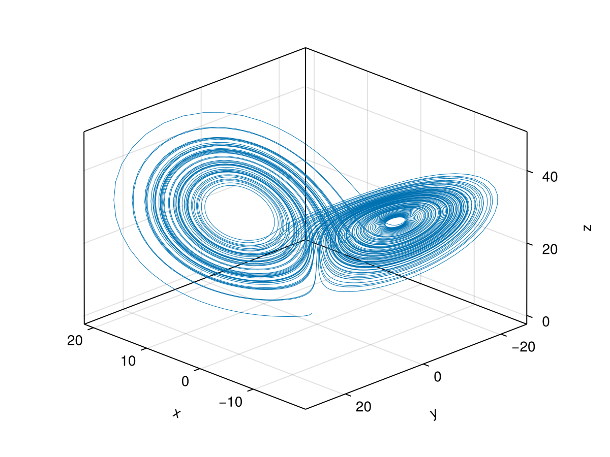
This is not clear what is going on because of the angle that we are viewing it. We can change that with the azimuth option of the Axis3 object. With a little bit of playing, if we do

🔗

fig = Figure()
ax = Axis3(fig[1,1], azimuth = 0.75pi)
lines!(ax, lorsol(t,idxs = 1).u, lorsol(t, idxs = 2).u, lorsol(t, idxs = 3).u, linewidth = 0.5)
fig

🔗

and this results in

🔗

For these examples, we have used the CairoMakie package for plotting. This is very nice for 2D plots (or projections of 3D plots into 2 dimensions), if we use the GLMakie package, we can get an interactive plot. First, we need to load and activate the package with

🔗

using GLMakie
GLMakie.activate!()
Makie.inline!(false)

🔗

and notice that we have set the inline to false so that the plot is not placed inside the notebook. And then run the plotting command with:

🔗

lines(lorsol(t,idxs = 1).u, lorsol(t, idxs = 2).u, lorsol(t, idxs = 3).u, linewidth = 0.5)

🔗

which should open up a window on your computer that allows you to rotate the plot with the mouse.

🔗

Subsection 43.4.2 Other Aspects of the `DifferentialEquations`

If you take a look at the the documentation of the package, we have only touched the surface of this package and it can do a lot with many different differential equations including initial value problems (that all three examples fit into), boundary value problems, stiff equations (aka they are hard to solve numerically) and stocastic differential equations.

🔗

Also, the actual solvers are not discussed here, however if you want to know the details, the documentation explains them. I have found that the default solvers are generally good enough and unless there is an issue, probably work for most problems.

🔗

Prev Top Next