Definition 18.1. Sample Space.
The sample space of an experiment is the set of all possible outcomes.
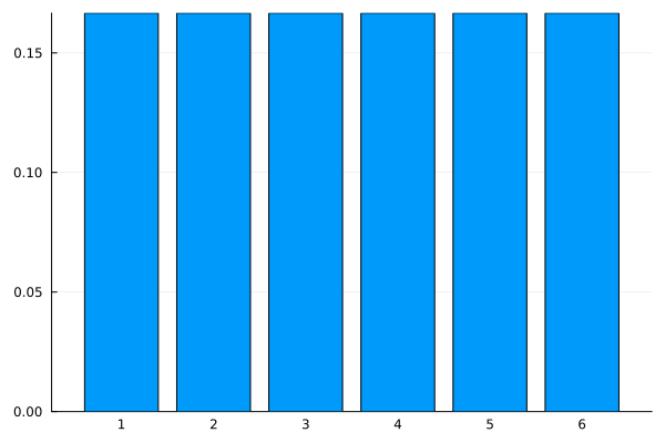
using Plots
bar(1:6, [1/6 for i=1:6], legend=false)
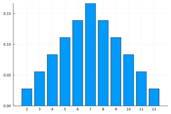
bar(2:12,[(6-abs(i-7))/36 for i=2:12], xticks=2:12, legend=false)


Random.seed! function.
using Random
Random.seed!(1234)
S=rand(1:6,10)
[2, 4, 2, 6, 3, 3, 6, 5, 3, 5] .
coins=rand(Bool,10)
[0, 0, 0, 1, 1, 0, 1, 0, 1, 0] This is a boolean Vector, note the Bool at the beginning. The 1s represent true and 0, false for compactness. Generally, as we did above, we will flip multiple coins and ask questions about the number of heads. We will examine this in the next chapter. If we are interested in unfair coin flips, we can choose randomly from an array where the unfair balance is known. For example,
rand([false,false,false,true,true],10)
[0 ,0 ,0 ,1 ,1 ,1 ,1 ,1 ,0 ,0] as a weighted coin where \(P(H)=2/5\) and \(P(T)=3/5\text{.}\)
S=rand(20)
20-element Vector{Float64}:
  0.3020595409518265
  0.05842018425830109
  0.20552381705814504
  0.7079246996200363
  0.41775698944882156
  0.22721762712581473
  0.7836312465908486
  0.20071380866783706
  0.6020380841683062
  0.5653680870733934
  0.7008893474454004
  0.4527965951678993
  0.13067526601187207
  0.4578870482605456
  0.6665192594508963
  0.5008741327606322
  0.8106990681415074
  0.46484850303763725
  0.9770123967639948
  0.5001612179097075
Distributions package in julia:
using Distributions
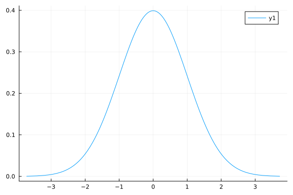
std_normal = Normal()
Normal{Float64}(μ=0.0, σ=1.0) and notice the mean and standard deviation are what we expect. Other means and standard deviations can be found by adding arguments. We can plot the normal distribution with
using StatsPlots
plot(std_normal)
random_normals = rand(std_normal,10)
10-element Vector{Float64}:
  2.121560382124172
 -0.26224077844309135
  0.3455010838287982
  0.44394906831563774
  0.44133351371484625
 -1.3397752732187238
  0.21507132788419303
  0.28927403687088354
 -0.6365687810422291
 -0.8196796137020412
Distributions package and the best place to start is at the Distributions package website