Numerical integration is a very important component of scientific computation. In tradition calculus classes, the integrals presented were ones that had antidervatives that could be found relatively easily. However, this is generally not true. For example, if trying to determine
the function \(f(x)=e^{-x^2}\) does not have an antidervative in terms of standard functions. This however it a very important antidervative in that it is related to the normal probability distribution. Because of its importance, we define
The trapezoid rule is one of the most basic numerical integration techniques. A geometric interpretation of numerical integration is to approximate the area under the curve with simpler known areas. In this case, we approximate the curve with a sequence of line segments which make trapezoids. A plot of the approximate integral of \(e^{-x^2}\) on the interval \([0,2]\) is given by
Let’s take a look at doing this in julia. To calculate the value we need a few things: 1) a function, 2) the interval we’re doing the approximation on and 3) the number of trapezoids or subintervals. We presented the following in Chapter 11 as
This is short and (maybe) sweet, but note that there are two separate arrays created. We have learned throughout this text, that the creation of arrays is often the most expensive part of a calculation. So instead, we will do the following:
function trapRule(f::Function, a::Real, b::Real; num::Int = 10)
  num > 0 || throw(ArgumentError("The number of trapezoids, num, must positive."))
  a < b || throw(ArgumentError("The left endpoint must be less than the right endpoint."))
  local h = (b-a)/num
  (h/2)*(f(a)+f(b)+2*sum(f,LinRange(a+h,b-h,num-1)))
end
Although this looks to be nearly the same, we haven’t created arrays. The LinRange function creates a range, but julia is savvy enough to not create the array to sum over it. See the exercise below. Let’s first redo the example above:
Use the BenchmarkTools and the @btime macro to compare the time of the trapezoid rule using the two functions shown here. Try integrating \(\sin(x^2)\) on \([0,1]\) for \(N=10,000\) subintervals.
The trapezoid rule uses straight lines to approximate the function and then integrates the line (or finds the area of the trapezoid). To find a better approximation if we use a quadratic function (parabola) to estimate the function. If we do this, then integrate the resulting parabola, this is called Simpson’s Rule. There are numerous places to find the derivation of this, but the result is
where \(h=(b-a)/n\text{,}\)\(x_k = a + kh\) and it is important that \(n\) is an even number. Similar to the trapezoid rule, we can write Simpson’s rule in julia as
function simpsonsRule(f::Function, a::Real, b::Real, n::Integer = 10)
  n > 0 || throw(ArgumentError("The number of subintervals, n, must be positive."))
  n % 2 == 0 || throw(ArgumentError("The number of subintervals, n, must be even."))
  a < b || throw(ArgumentError("The left endpoint must be less than the right endpoint."))
  local h = (b-a)/n
  xpts = LinRange(a,b,n+1)
  (h/3)*(f(a)+f(b) + 4*sum(f,xpts[2:2:end-1]) + 2*sum(f,xpts[3:2:end-2]))
end
Applying Simpson’s Rule to \(\int_0^3 x^2 \, dx\) as
It’s interesting to note that this reports the exact value. In fact, Simpson’s rule will numerically integrate any cubic (and lines and quadratics) exactly. If we return to trying to find \(\int_0^2 e^{-x^2} \, dx\) and use Simpson’s Rule, then
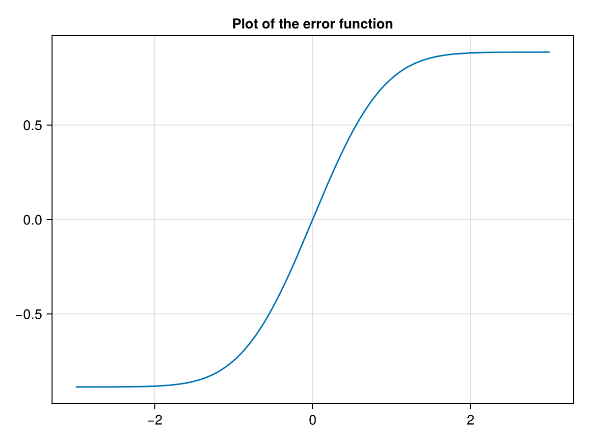
We can use numerical integration to evaluate the error function at any value, so let’s go ahead and plot it. First, let’s make a function that defines the error function.
function erf(x::Real)
  local area = simpsonsRule(t -> exp(-t^2),0,abs(x),100)
  x > 0 ? area : -1*area
end
where we have used the symmetry of the error function to evaluate it if x is positive or negative. If we don’t check for this, we will get an error because simpsonsRule has a check that the interval needs to be put in as \(a < b\text{.}\) Now, we can plot it with: