Chapter 38 Analyzing Census Data
This chapter goes through an example of analyzing census data. We load the data then ask a number of questions of the data. It is expected that you have read Chapter 31 and Chapter 35 before this.
Section 38.1 Loading Packages and the Dataset
Before we begin, make sure that you have added and loaded the following packages:
using DataFrames, Chain, Statistics, CSV, StatsPlots
Download the file Gaz_ua_national.csv and save it somewhere that you can access it from Julia. This file has a lot of census data that we will try to find answers. Information about the data is on the census website
For this chapter we will need load the packages
DataFrames, Chain, Statistics, CSV and will start by loading the file with
census = CSV.read("Gaz_ua_national.csv",DataFrame)
or adjusting the path to the file if needed.
Section 38.2 Answering Census Questions
There are a number of questions that we can answer. We will spend the rest of this chapter answer these questions.
-
What is the total population of all areas?
-
What are the top 10 areas in population?
-
How many population areas are west of 120 degrees longitude?
-
Give a histogram plot in terms of population?
-
What is the total number of housing units?
-
What the top 10 area in housing units?
-
What are the top 10 areas in land size?
-
What are the top 10 areas in water size?
-
List the top 5 Massachusetts areas by population.
-
What is the average population, median and standard deviation of all Massachusetts areas?
Subsection 38.2.1 Data Analysis of Census Data
Now that we have the data loaded and stored in the DataFrame called
census, there are a number of ways to answer the questions posed above. A nice clean technique is to answer the question by building a @chain block that starts with the census DataFrame and results in the answer. Most of the time this works and we will show this in the rest of the chapter. For complicated questions, we will walk through step by step how to do this.
Subsection 38.2.2 What is the total population of all areas?
@chain census begin
  combine(:POP10 => sum => :TOTAL_POP)
end
which returns
1×1 DataFrame
Row  TOTAL_POP
     Int64
1    252746527
indicating that the total population is 252746527. Note: the total U.S. Population in 2010 was about 309 million, so this dataset is not capturing everyone.
Subsection 38.2.3 What are the top 10 areas in population?
To solve this, we will start with the data frame and take only necessary columns, sort by the
POP10 column and print out the top 10 rows. We will build up these steps within a @chain block:
@chain census_data begin
  select(:NAME, :POP10)
  sort(:POP10, rev = true)
  first(10)
end
and this returns
10×2 DataFrame
Row  NAME                                                 POP10
     String                                               Int64
1    New York--Newark, NY--NJ--CT Urbanized Area          18351295
2    Los Angeles--Long Beach--Anaheim, CA Urbanized Area  12150996
3    Chicago, IL--IN Urbanized Area                        8608208
4    Miami, FL Urbanized Area                              5502379
5    Philadelphia, PA--NJ--DE--MD Urbanized Area           5441567
6    Dallas--Fort Worth--Arlington, TX Urbanized Area      5121892
7    Houston, TX Urbanized Area                            4944332
8    Washington, DC--VA--MD Urbanized Area                 4586770
9    Atlanta, GA Urbanized Area                            4515419
10   Boston, MA--NH--RI Urbanized Area                     4181019
Subsection 38.2.4 Find the total population of the areas west of 120 degrees longitude?
The number of degrees longitude is in the column
INTPTLONG and is a negative number because it is west of the 0 degree longitude (that’s the way it works). West of 120 degrees is less than -120.
We will filter (subset) the data frame using this and then
combine to compute the sum.
@chain census begin
  subset(:INTPTLONG => long -> long .< -120)
  combine(:POP10 => sum => :POP_WEST_120)
end
The result is
1×1 DataFrame
Row  POP_WEST_120
     Int64
1    21932350
The result shows the total population west of 120 degrees is about 22 million.
Subsection 38.2.5 Give a histogram plot in terms of population?
To produce a histogram of the population, we will use the
hist method from the Makie package. Check out the documentation. If we do:
hist(census.POP10)
then we get the following plot:
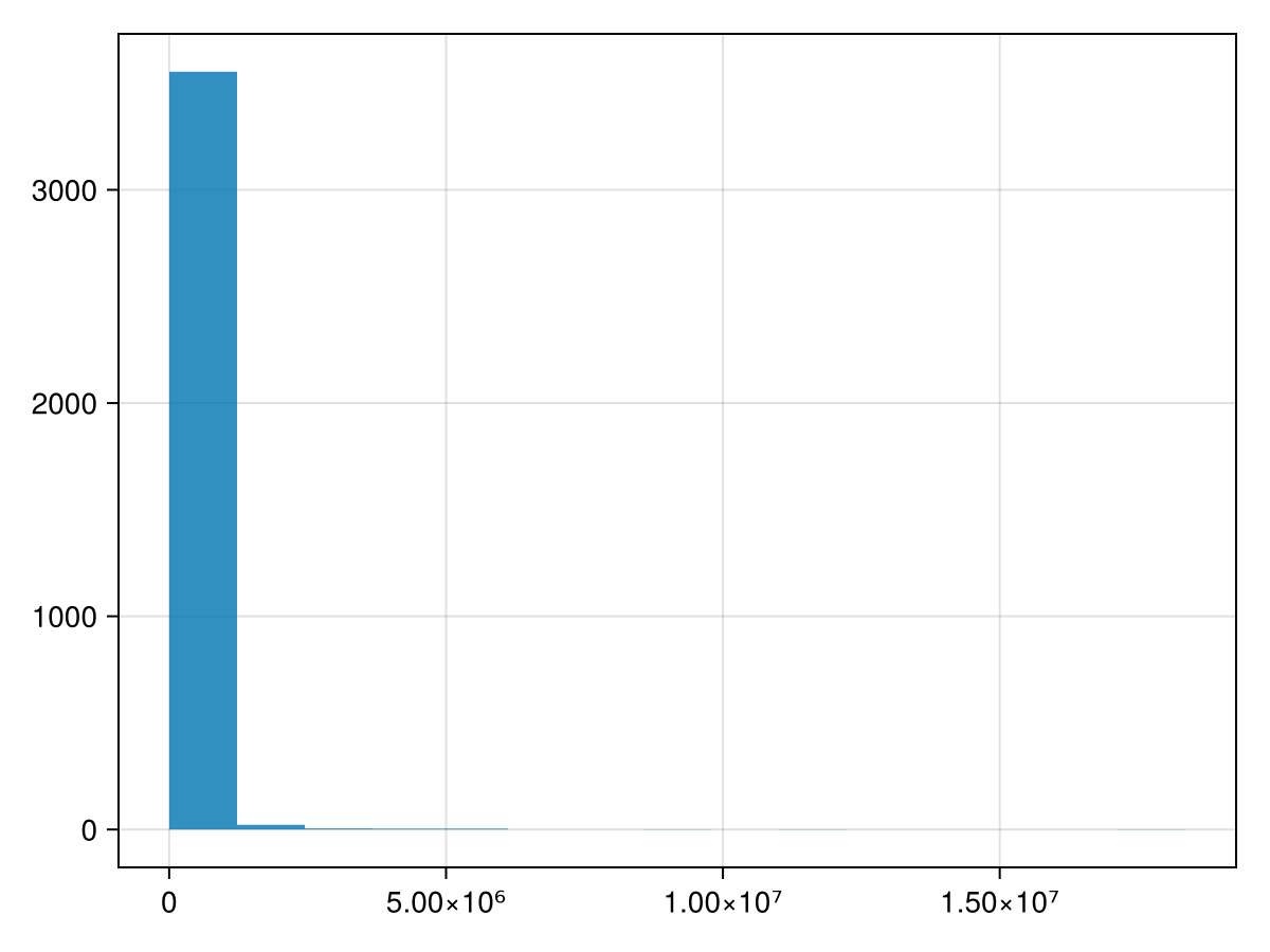
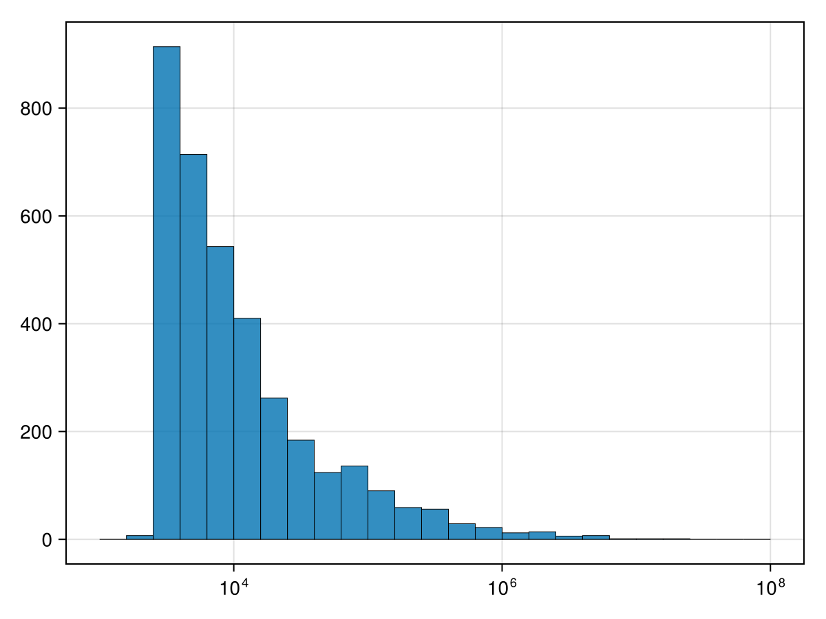
The trouble with this is that there are many many census areas with very little population. We can fix this with a log scale. If you enter
b=10 .^(3:0.2:8)
fig = Figure()
ax = Axis(fig[1,1], xscale = log10)
hist!(ax, census.POP10, bins=b, strokewidth=0.5)
fig
where the
b variable is the locations of the bin boundaries. This took some experiments to get the right sizes. The attribute xscale sets the scale to base-10 logarithmic scale.
then the result is:
Subsection 38.2.6 What the top 10 area in housing density?
We are interested in finding the highest housing density, that is the number of people per housing units. We will create a new column to do this:
@chain census begin
  transform( [:POP10, :HU10] => ((p,h)-> p./h) => :Housing_Density)
  select(:NAME, :Housing_Density)
  sort(:Housing_Density, rev=true)
  first(10)
end
the results of this is
10×2 DataFrame
Row   NAME                                   Housing_Density
      String                                 Float64
1     Air Force Academy, CO Urban Cluster    16.908
2     Colorado City, AZ--UT Urban Cluster     8.1839
3     Kinross, MI Urban Cluster               6.75773
4     Soledad, CA Urban Cluster               6.61642
5     Alfred, NY Urban Cluster                6.55842
6     Avenal, CA Urban Cluster                6.44713
7     Corcoran, CA Urban Cluster              6.12188
8     Montgomery, PA Urban Cluster            5.83454
9     Darbydale, OH Urban Cluster             5.6216
10    Woodville, FL Urban Cluster             5.37327
Subsection 38.2.7 What is the total number of housing units?
This is simply a summary statistic on the
HU10 variable:
@chain census begin
  combine(:HU10 => sum)
end
which has the result
105549535.
Subsection 38.2.8 What are the top 10 areas in land size?
This is a sorting of the dataset in terms of the
ALAND variable:
@chain census begin
  select(:NAME, :ALAND)
  sort(:ALAND, rev=true)
  first(10)
end
and the result is
10×2 DataFrame
Row  NAME                                                 ALAND
     String                                               Int64
1    New York--Newark, NY--NJ--CT Urbanized Area          8935981360
2    Atlanta, GA Urbanized Area                           6851428985
3    Chicago, IL--IN Urbanized Area                       6326686332
4    Philadelphia, PA--NJ--DE--MD Urbanized Area          5131721516
5    Boston, MA--NH--RI Urbanized Area                    4852227548
6    Dallas--Fort Worth--Arlington, TX Urbanized Area     4607936452
7    Los Angeles--Long Beach--Anaheim, CA Urbanized Area  4496266014
8    Houston, TX Urbanized Area                           4299420988
9    Detroit, MI Urbanized Area                           3463234750
10   Washington, DC--VA--MD Urbanized Area                3423261150
Subsection 38.2.9 What are the top 10 areas in water size?
This is similar to the one above but use the
AWATER variable:
@chain census_data begin
  select(:NAME, :AWATER)
  sort(:AWATER, rev=true)
  first(10)
end
and the result is
10×2 DataFrame
            Row  NAME                                          AWATER
                 String                                        Int64
            1    New York--Newark, NY--NJ--CT Urbanized Area   533176599
            2    Minneapolis--St. Paul, MN--WI Urbanized Area  232127029
            3    Tampa--St. Petersburg, FL Urbanized Area      211394181
            4    Boston, MA--NH--RI Urbanized Area             201870511
            5    Jacksonville, FL Urbanized Area               199369291
            6    Miami, FL Urbanized Area                      191964476
            7    Virginia Beach, VA Urbanized Area             189979138
            8    Seattle, WA Urbanized Area                    173839079
            9    Orlando, FL Urbanized Area                    142321970
            10   Palm Bay--Melbourne, FL Urbanized Area        130390065
Subsection 38.2.10 List the top 5 Massachusetts areas by population.
First, we’ll need to filter (subset) the dataset to only include those with
MA in the name. We can use the occursin function to do this:
  @chain census begin
  subset(:NAME => (n -> occursin.("MA",n)))
  sort(:POP10, rev= true)
  first(5)
  select(:NAME, :POP10)
end
and the result is:
5×2 DataFrame
Row  NAME                                POP10
     String                              Int64
1    Boston, MA--NH--RI Urbanized Area   4181019
2    Providence, RI--MA Urbanized Area   1190956
3    Springfield, MA--CT Urbanized Area  621300
4    Worcester, MA--CT Urbanized Area    486514
5    Barnstable Town, MA Urbanized Area  246695
Subsection 38.2.11 What is the average population, median and standard deviation of all Massachusetts areas?
This is similar to above, except we change the functions on the combine:
@chain census_data begin
  subset(:NAME => (n -> occursin.("MA",n)))
  combine(:POP10 => mean, :POP10 => median, :POP10 => std)
end
which results in
1×3 DataFrame
Row  POP10_mean  POP10_median  POP10_std
     Float64     Float64       Float64
1    3.69408e5   20717.5       9.44398e5
