Chapter 49 Working with a weather web API and JSON strings
This chapter will shown how to interact with a web API, a common way of getting data from a webserver in a way that can be more easily processed than with a HTML page. We first start with what a JSON string is and how to parse it, recall some basics of dictionaries from Section 22.3 and then make API calls using some network tools in Julia.
Section 49.1 JSON Strings
A JSON string is a robust way of storing data as a single string. It stands for Javascript Object Notation and is the most ubiquitous way of passing data between webservers or often between a webserver and a client. The following is an example of something we saw in Section 22.3
str = """
{
  "first_name": "Homer",
  "last_name": "Simpson",
  "age":45,
  "phones": [
    {"number": "987-555-1234", "type": "home"},
    {"number": "987-555-1212", "type": "cell"}
  ],
  "home_address": {
    "street": "742 Evergreen Terrace",
    "city": "Springfield"
  },
  "work_address": {
    "street": "10 Power Plant Lane",
    "city": "Springfield"
  }
}
"""
Recall that a multiline string in Julia starts and ends with triple double quotes
""". The rest of it looks like a Dictionary and that is the type of object we will get when parsing the string.
A few things to note is that an object with key-value pairs are surrounded by curly (squiggly) braces
{} and similar to Julia arrays are square brackets like []. Notice that all strings must be surrounded by double quotes and the key value pairs are separated by a colon (:).
Let’s say that this string was sent by a webservice and you need to do something to the object (perhaps display its results in a nice format). The first thing to do is to parse the string using the
JSON package. Make sure you have downloaded it and are using JSON.
We parse it with the
JSON.parse method as in h = JSON.parse(str) and you should see something similar to
Dict{String, Any} with 6 entries:
  "first_name"   => "Homer"
  "home_address" => Dict{String, Any}("city"=>"Springfield", "street"=>"742 Eve…
  "phones"       => Any[Dict{String, Any}("number"=>"987-555-1234", "type"=>"ho…
  "work_address" => Dict{String, Any}("city"=>"Springfield", "street"=>"10 Powe…
  "last_name"    => "Simpson"
  "age"          => 45
where some of the longer values are cutoff with the
… at the end of the line. Parsing with the JSON package will also result in a Dictionary and you may need to refresh your memory in Section 22.3. For example, you can get the first name of this person with
h["first_name"]
Rarely does a programmer write JSON. Instead, JSON is generated by encoding objects to strings using methods. In general, encoding an object to be stored or transfered is called serialization. Another example might be that we have a menu stored as a Dictionary. For example,
menu = Dict("items" => [
  Dict("name" => "hamburger", "type" => "sandwich", "price" => 10.99),
  Dict("name" => "Club Sandwich", "type" => "sandwich", "price" => 12.99),
  Dict("name" => "spaghetti", "type" => "main", "price" => 14.99),
  Dict("name" => "Caeasar Salad", "type" => "salad", "price" => 7.99),
  Dict("name" => "Chococate Ice Cream", "type" => "dessert", "price" => 6.99),
])
creates a dictionary to store a menu. We can encode this as a JSON string with
JSON.json(menu) and this returns
"{\"items\":[{\"name\":\"hamburger\",\"price\":\"10.99\",\"type\":\"sandwich\"},{\"name\":\"Club Sandwich\",\"price\":\"12.99\",\"type\":\"sandwich\"},{\"name\":\"spaghetti\",\"price\":\"14.99\",\"type\":\"main\"},{\"name\":\"Caeasar Salad\",\"price\":\"7.99\",\"type\":\"salad\"},{\"name\":\"Chococate Ice Cream\",\"price\":\"6.99\",\"type\":\"dessert\"}]}"
and notice that it comes back with no line breaks. JSON isn’t designed to be easily readable. Instead, it is designed to compactly store data. However, there is a package called
PrettyPrint that allows better printing. Download and do using PrettyPrint and then
Section 49.2 Handling Files
As we discussed, JSON is a format that is generally used to transfer data between computers. Instead of it being typed in, it will often be stored as a file, and will be helpful to review Chapter 27. Later, we use a command to save a file and another to read it, however it is helpful to understand file structure offered in that chapter.
Section 49.3 Querying a Geocoding Service
In this section we will query a geocoding service offering from the census bureau in order to translate a location (town name) or address to a latitude and longitude. The information on the service and how access it is found at this Census Bureau website. We will show some examples using Julia here.
In general, the service is available in the form:
https://geocoding.geo.census.gov/geocoder/returntype/searchtype?parameters
where
returntype is either locations or geographies and searchtype is onelineaddress OR address OR addressPR OR coordinates and will be shown in examples below.
To make a call using Julia, we will use the
Downloads.request method and to use this you must first load the Downloads module by entering using Downloads. Note: Downloads is a built-in module, so you don’t need to add it via the package manager, but will need to add it to the namespace.
As an example, we will get information of the TD garden (home of the Boston Bruins and Boston Celtics) by the following url
url = "https://geocoding.geo.census.gov/geocoder/locations/address?street=80+Causeway+St&city=Boston&state=MA&zip=02114&benchmark=4&format=json"
Downloads.request(url, output = "tdgarden.json")
Which makes a request to the webserver at
https://geocoding.geo.census.gov with the given address and other parameters. Note that the output is saved in a file called "tdgarden.json". Go ahead and look at it in VS code or another text editor, however JSON files are generally a good method for sending data between computers and is not very readable.
We will load in the json file with the command
j = JSON.parsefile("tdgarden.json") and then pretty printing it with pprintln(j) results in
        {
  "result" : {
               "addressMatches" : [
                                    {
                                      "tigerLine" : {"side" : "L",
                                                     "tigerLineId" : "85709714"},
                                      "coordinates" : {"x" : -71.063299192963,
                                                       "y" : 42.364398683584},
                                      "addressComponents" : {"toAddress" : "50",
                                                             "preQualifier" : "",
                                                             "zip" : "02114",
                                                             "state" : "MA",
                                                             "preType" : "",
                                                             "streetName" : "CAUSEWAY",
                                                             "suffixType" : "ST",
                                                             "preDirection" : "",
                                                             "city" : "BOSTON",
                                                             "suffixQualifier" : "",
                                                             "suffixDirection" : "",
                                                             "fromAddress" : "98"},
                                      "matchedAddress" : "80 CAUSEWAY ST, BOSTON, MA, 02114",
                                    },
                                  ],
               "input" : {
                           "benchmark" : {"benchmarkName" : "Public_AR_Current",
                                          "isDefault" : true,
                                          "benchmarkDescription" : "Public Address Ranges - Current Benchmark",
                                          "id" : "4"},
                           "address" : {"city" : "Boston",
                                        "zip" : "02114",
                                        "street" : "80 Causeway St",
                                        "state" : "MA"},
                         },
             },
}
Recall that the desire in this API call was to get the longitude and latitude coordinates of the location. This is on lines 7 and 8 of the above outuput, but can be accessed from the Dictionary with
j["result"]["addressMatches"][1]["coordinates"]
which returns
Dict{String, Any} with 2 entries:
  "x" => -71.0633
  "y" => 42.3644
Section 49.4 Accessing API Weather Data
The previous example was relatively simple and this will give a more complex example. We will use the service from
openweathermap.org to access weather data for a particular location. First, you should visit the site and create an account (for free) to access an API key. This will be needed below.
After signing up, go to ???? to access your API key and make a note of it (or store it in a file on your personal computer. )
We will make a call to get a 4-day/3-hour forecast for Fitchburg, MA. First, use the service above to get the coordinates (I used the address of 100 Main Street in Fitchburg) and received
-71.793 for the longitude and 42.5817 for the latitude.
This is then fed into the openweather API as
Downloads.request("https://pro.openweathermap.org/data/2.5/forecast?lat=42.5817&lon=-71.793&units=imperials&appid=5a6e6bf61f0f285da7a9886694c04c87", output = "weather.json")
The weather data is then stored in the file
"weather.json". Also, the units used was changed from standard to imperial the units used in the United States. We can parse the JSON file with
weather = JSON.parsefile("weather.json")
and examine the results with
pprintln(weather). You will see that it is a large file. The main weather information is in the list field and the next step is to extract the data and place this in a DataFrame. Although there is a lot of information there, we will extract the time, temperature, humidity, wind and conditions from this to begin with. First, we will make an empty DataFrame with these columns with the following command:
weather_df = DataFrame(time = Int[], temp = Float64[], humidity = Int[], wind = Float64[], conditions = String[])
Extracting the correct data requires that the proper fields are included. All of the desired data is in the
"list" field, which is an array of other data, so for each element of this, we extract the time, temp, wind, ... First, let’s just show the conditions with
for w in weather["list"]
  weath =  (time = w["dt"], temp = w["main"]["temp"], humidity = w["main"]["humidity"], wind = w["wind"]["speed"], conditions = w["weather"][1]["main"])
  @show weath
end
but the output is not shown here, but it appears that it was parsed correctly. To add this to the dataframe, we change the above to
for w in weather["list"]
  append!(weather_df, [(time = w["dt"], temp = w["main"]["temp"], humidity = w["main"]
  ["humidity"], wind = w["wind"]["speed"], conditions = w["weather"][1]["main"])])
end
weather_df
And the result of this should be similar to
40×5 DataFrame15 rows omitted
Row	time	temp	humidity	wind	conditions
Int64	Float64	Int64	Float64	String
1	1734102000	24.17	61	10.18	Clear
2	1734112800	25.83	52	11.3	Clear
3	1734123600	25.32	50	8.79	Clear
4	1734134400	24.28	56	6.44	Clear
5	1734145200	23.18	60	6.26	Clear
6	1734156000	22.37	66	5.59	Clear
7	1734166800	21.29	66	4.0	Clear
8	1734177600	20.32	67	3.36	Clear
9	1734188400	27.16	42	6.53	Clear
10	1734199200	31.28	31	6.06	Clear
11	1734210000	26.87	47	4.23	Clear
12	1734220800	23.56	62	2.86	Clear
13	1734231600	22.73	67	2.53	Clear
⋮	⋮	⋮	⋮	⋮	⋮
29	1734404400	39.88	99	5.73	Clouds
30	1734415200	45.81	97	10.67	Rain
31	1734426000	47.59	94	11.72	Rain
32	1734436800	51.42	92	15.46	Clouds
33	1734447600	52.45	94	13.4	Rain
34	1734458400	52.65	90	14.5	Rain
35	1734469200	48.51	86	14.63	Rain
36	1734480000	38.66	81	10.71	Clouds
37	1734490800	37.58	84	12.39	Clouds
38	1734501600	36.18	85	10.18	Clouds
39	1734512400	35.33	83	9.86	Clouds
40	1734523200	32.65	91	4.94	Clouds
The units for the
time column is given in unix time, the number of seconds since January 1, 1970. On the surface this seems to be a strange way to measure time, but many things (like time differences and time zones) can be handled relatively easily. The units of the other columns are standard for temperature (Fahrenheit) and wind speed (miles per hour). The site https://openweathermap.org/forecast5 gives additional details about each of the fields and the units.
Although there is much we can do with the time data, we will just make a simple new column that represents the number of hours since the beginning of the forecast (first row of data). Since this is in seconds, we will first shift by the unix time of the first row and then divide by 3600 (number of seconds in an hour). This can be done using the
@chain blocks shown in Chapter 35 as
weather2 = @chain weather_df begin
  transform(:time => (t-> (t .- 1734102000 )/3600) => :time_hours)
end
The results add a new column called
time_hours to the DataFrame which is the number of hours into the forecast, which runs from 0.0 to 117.0.
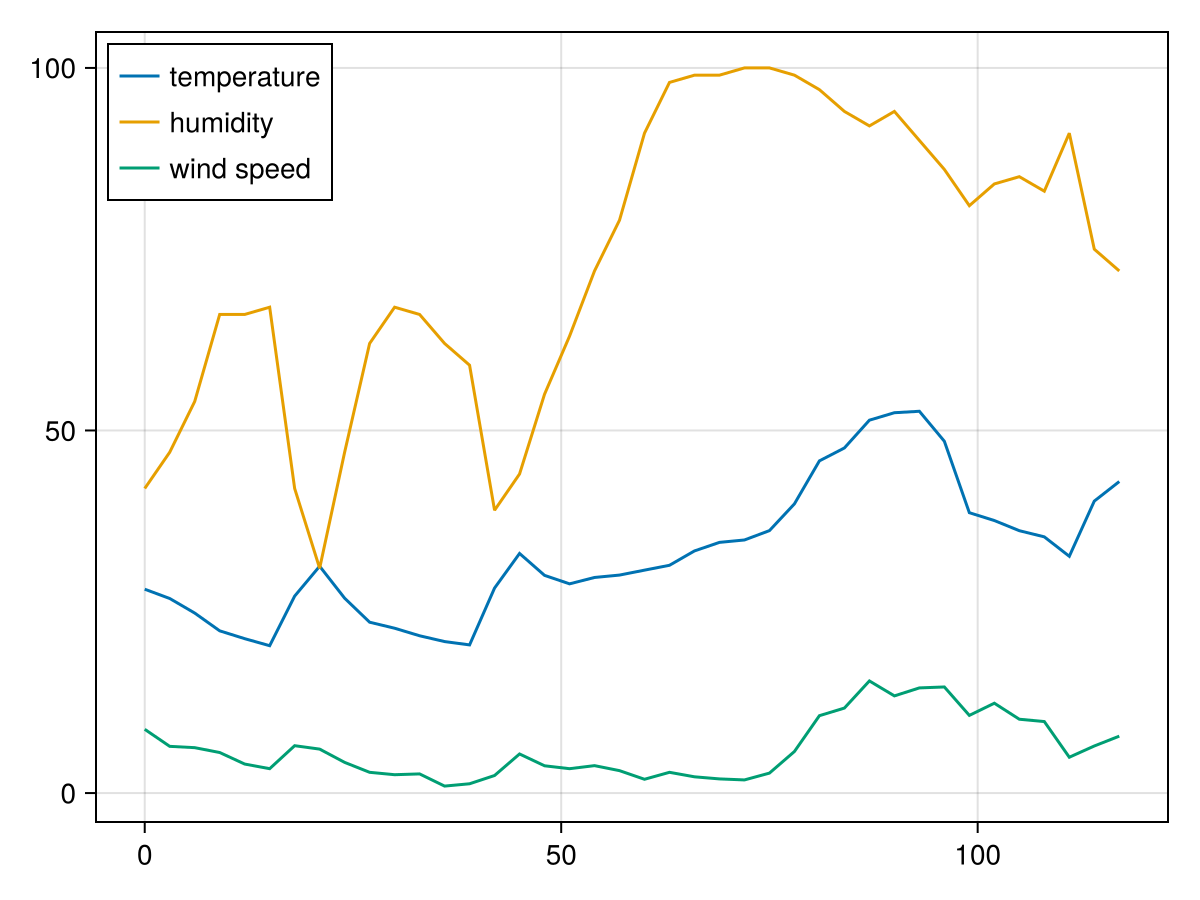
We can plot of the data above using techniques in Chapter 14, Chapter 15 and Chapter 32. In this example, we will make line plots with
time_hours on the horizontal and temp, humidity and wind as separate plots using the following code:
fig, ax = lines(weather2.time_hours, weather2.temp, label = "temperature")
lines!(ax,weather2.time_hours, weather2.humidity, label = "humidity")
lines!(ax,weather2.time_hours, weather2.wind, label = "wind speed")
axislegend(ax, position = :lt)
fig
and when I downloaded the data, the plot I got was: