Chapter 13 Plotting Basics
Plotting is an important aspect of anything scientific or mathematical. The ability to visualize a complex model or data set is often key to understanding it. In Julia, there are two different systems currently that are both used. These are called Makie and the Plots package.
Also, as is common with open systems, like Julia, both Makie and Plots are user-developed systems that are evolving separate from each other. Both have advantages and philosophies associated with them. We will cover them each in depth in the next two chapters.
Section 13.1 Introduction to Makie
On the official Makie Home Page: Makie is a data visualization ecosystem for the Julia programming language, with high performance and extensibility.
There is definitely a philosophy of making attractive plots in Makie. In fact, there is another website called Beautiful Makie whose purpose is to show off the amazing plots. The following is an example of a combination surface and vector field plot
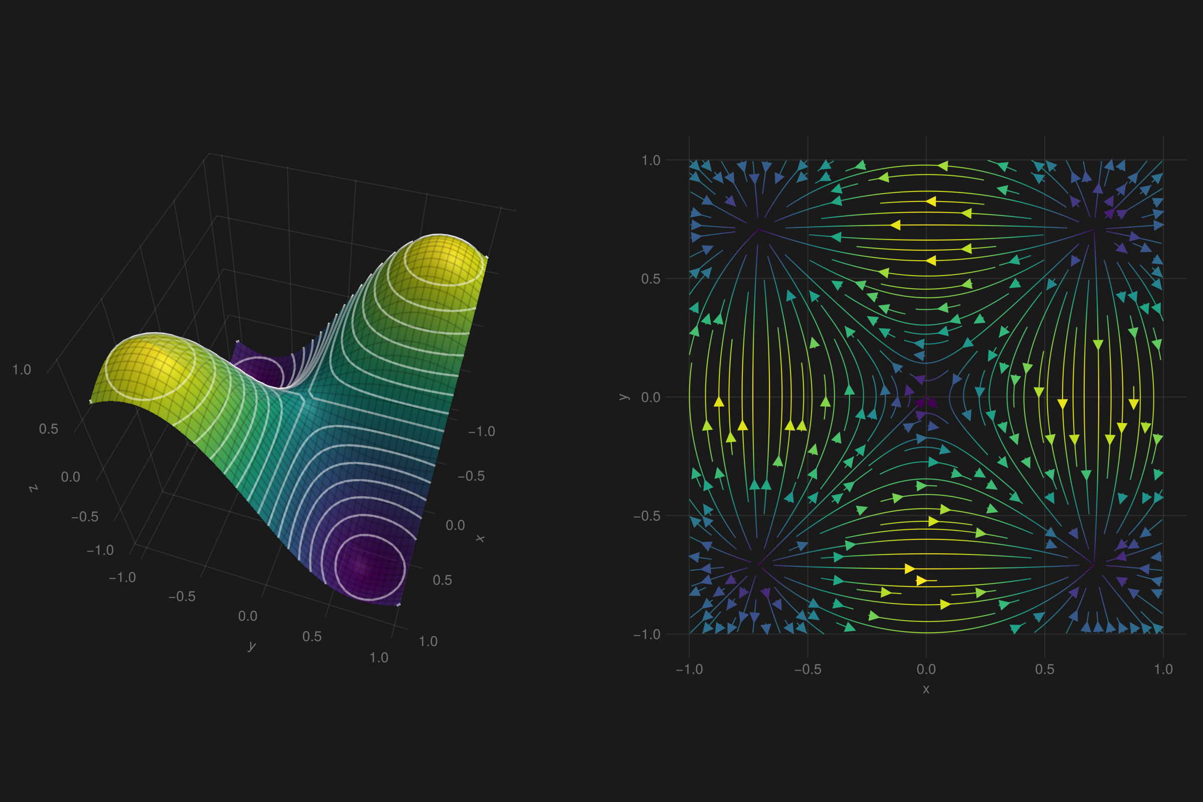
I won’t post the code here, but it is available at the Beautiful Makie website. However, it is about 20 lines of code, which is quite compact for such a plot.
Section 13.2 Introduction to the Plots package
Plots is a packaging system that has some similar ideas to that of Makie. According to the Plots website, the goals with the package are:
-
Powerful. Do more with less. Complex visualizations become easy.
-
Intuitive. Start generating plots without reading volumes of documentation. Commands should "just work."
-
Concise. Less code means fewer mistakes and more efficient development and analysis.
-
Flexible. Produce your favorite plots from your favorite package, only quicker and simpler.
-
Consistent. Don’t commit to one graphics package. Use the same code and access the strengths of all backends.
-
Lightweight. Very few dependencies, since backends are loaded and initialized dynamically.
-
Smart. It’s not quite AGI, but Plots should figure out what you want it to do... not just what you tell it.
An example of using Plots is the following Lorenz attractor as an animator. If you return to the Makie Homepage, you’ll see a similar example.
Section 13.3 Plotting is Hard
Why is plotting hard? Often plotting is what takes the most CPU/GPU cycles in a project. In fact, the team of developers that have been working on Julia have given this issue the acronym TTFP (time to first plot), which is the amount of time from starting Julia to getting a plot rendered. Recently a lot of work has been done to reduce this.
When people usually think of plots or visualization, we think of high-level ideas, like function plots, scatter plots, vector field plots, etc. We’d like to give functions or data and some attributes to some plotting routine and then just wait for the results. These routine need to handle a lot of the details, including drawing lines and points on the screen with various fonts and make sure that all of the spacing is correct.
Section 13.4 Presenting Results with Visualization, an overview
Before starting with code to create plots, let’s remind ourselves of the types of plots that can occur and what they mean.
Subsection 13.4.1 Scatter Plots
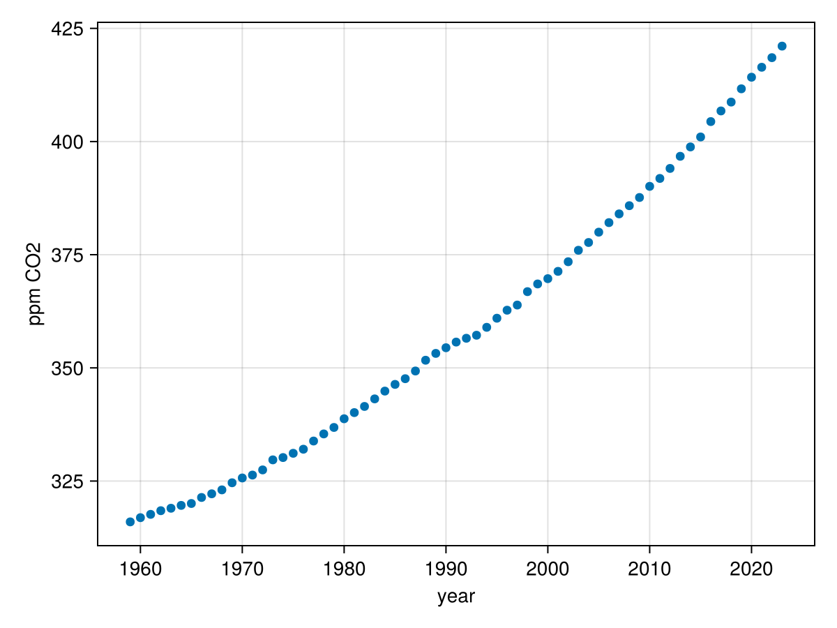
A scatter plot is a plot of points in 2D or 3D in which each point represents a piece of data. Although we will usually think of them in terms of x, y and z axes, the two or three axes can represent anything. The following is the graph of carbon dioxide levels in Hawaii from 1959 to 2023.
Subsection 13.4.2 Function Plots
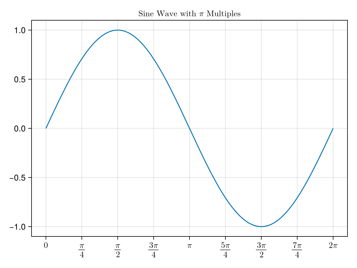
Mathematically, the graph of a function \(f(x)\) is the set of all points that satisfy the points \((x,f(x))\) or if it is a function of two variables \((x,y,f(x,y))\text{.}\) This is generally what is thought of as a function graph that is often first seen in a Precalculus class, but extends throughout a science fields. The following is a sine curve.
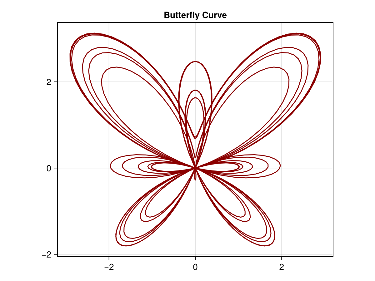
Subsection 13.4.3 Parametric Plots
Additionally, a function plot can be created for a parametric curve defined as \(\langle x(t), y(t) \rangle \) for functions \(x\) and \(y\text{.}\) A very nice example is that of the butterfly curve:
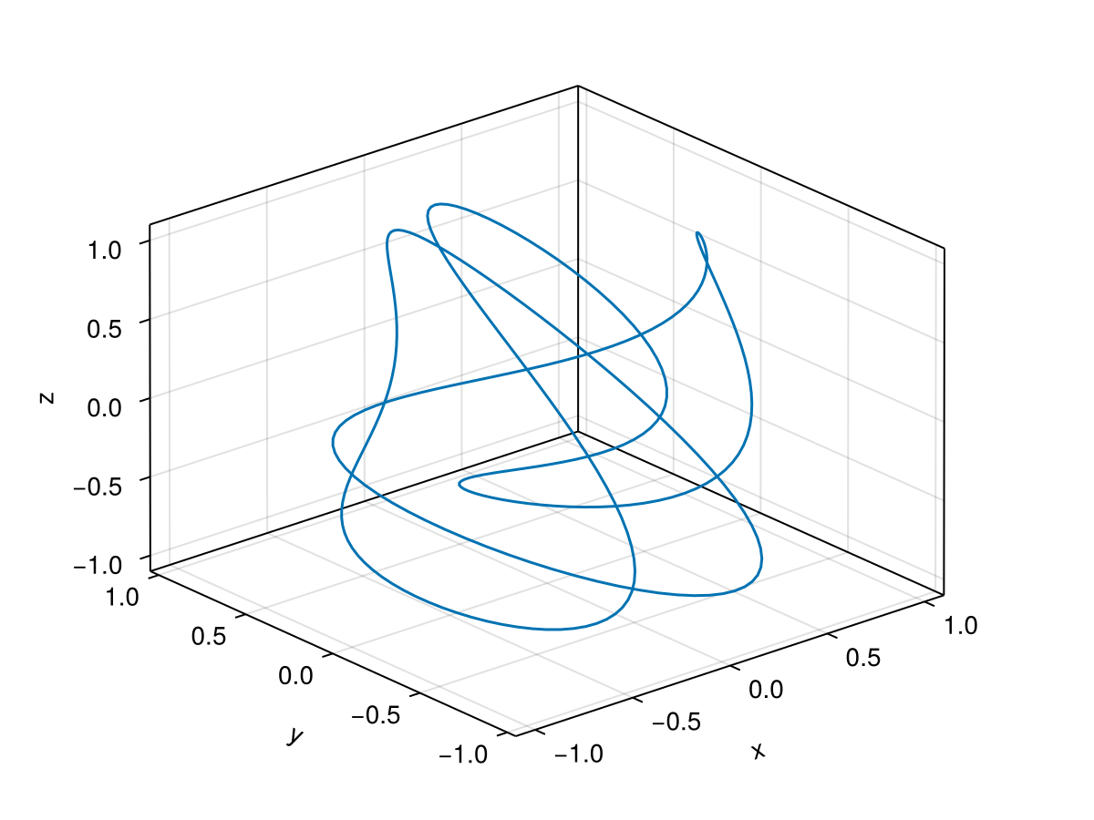
Subsection 13.4.4 Parametric Plots in 3D
Vector Functions in 3D are often represented as parametric functions of the form:
\begin{equation*}
\langle x(t), y(t), z(t) \rangle
\end{equation*}
where each function gives the \(x\text{,}\) \(y\) or \(z\) coordinate at a time \(t\text{.}\) An example of this is the parametric function \(\langle \cos 2t \cos t, \cos 5t \cos t, \sin 3t \rangle\text{.}\)
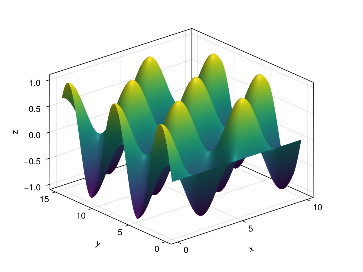
Subsection 13.4.5 Surface Plots
Functions of two variables in the form \(z = f(x,y)\) and that the two independent variables are \(x\) and \(y\) and the third variable is the height of the function. The set of points that satisfy this equation generally form surfaces in 3D. An example of this is the function \(f(x,y)=\sin x \cos y\) which has the surface plot
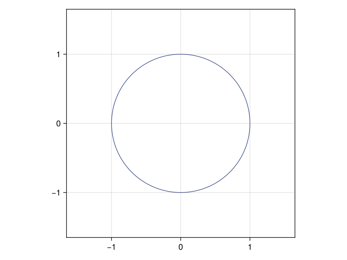
Subsection 13.4.6 Implicit Curves
An implicit curve is the set of points \((x,y)\) in which \(f(x,y)=C\) for some constant \(C\text{.}\) The classic example is the circle
\begin{equation*}
x^2 + y^2 = 1
\end{equation*}
The following is the circle above plotted implicitly:
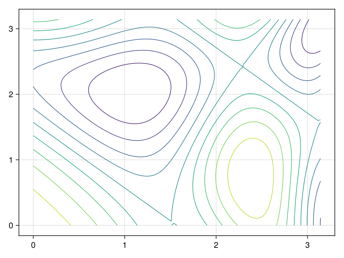
Subsection 13.4.7 Contour Plots
Related to plots of an implicit curve is that of a contour plot. Recall from above that a function of two variables \(z=f(x,y)\) can be plotted in 3D, however another way to view these is as a series of implicit curves in the form \(f(x,y)=C\) for some number of constants \(C\text{.}\) For example, the contour plot of
\begin{equation*}
f(x,y) = \sin\left(\frac{1}{2}x^2-\frac{1}{4}y^2+2\right)\cos(x+y)
\end{equation*}
has the contour plot:
Section 13.5 Plotting Backends
Each of the two plotting environments that we are discussing in this chapter rely on other software to do the plotting. These are known as backends, which are the actual routines to draw the lines, place the glyphs in a font and handling spacing. There is different technology that is used for each backend and you don’t need to know the specifics, but you should know that there are different backends and there are strengths and weaknesses of each.
Makie and the Plots package are each high-level wrappers with a consistent interface. That is, say, to perform a function plot, each takes a function, the limits and various attributes of the plot and the backends handle the details. Although we haven’t discussed which plotting environment to use, one way to decide is which style of wrappers do you like better.
As this text is agnostic for the plotting environment, once that is chosen, some reading should be done on the backend. Each of the next two chapters covers the backends for Makie and Plots respectively.
