Solving an equation is something that is needed throughout scientific computing and is difficult to do in general. For example, if we have an equation like \(x^2-1=0\text{,}\) this can be solved exactly using the quadratic formula, however the relatively simple equation \(x=\sin(x)\) has no analytic solution. In this chapter, we discuss how to find roots of both quadratic functions and general functions, but also use this to discuss both errors in a algorithm as well as round off error, which occurs often when solving problems.
The definition about saying that a root is a value where \(f(x)=0\) and an equation like \(x=\sin(x)\) doesn’t fit this form, but recall that the equation can be algebraically manipulated to get to be a root as \(f(x) = x-\sin(x)\) or \(f(x)=\sin(x) -x\text{.}\)
Consider an algorithm that tries to find the value of \(x^{\star}\text{.}\) In general, an algorithm won’t return the value \(x^{\star}\) but a value \(x\) that is close, therefore there will be some error. The absolute error is \(|x - x^{\star}|\) and the relative error is
We are going to solve this using the quadratic formula in Julia. To study rounding effects we’re going to solve these using both 16-bit and 64-bit floating point numbers. We’ll assume that the 64-numbers are the actual answers in determining errors.
Use the quadratic formula to solve \(2.56632x^{2}+ 17.34x+ 0.01734=0\) using both BigFloats and 64-bit floats. Assume that the BigFloat versions are exact and find the absolute and relative errors in the 64-bit numbers.
Even though the example above was manufactured to produce bad results, you never know if a numerical solution is accurate or not. One way to look at the above example is to not use 16-bit floating point numbers. This is a good idea, but assume (like we did above) that 64-bit is the actual answer. There are cases where you will get the wrong answer with 64-bit.
It’s crucial to have a good sense of the problem (whether it be mathematical or a scientific question). Additionally, testing is an important part of the solution process. In Chapter 23, we will spend some time discussing testing of code.
Section10.3Are We Sunk? Reexamining the Quadratic Formula
The above example shows that even with a well-known formula, there is the potential of generating a large error. From what we’ve seen so far, we could try to use other data types, like BigFloat to solve this problem, but as we’ve seen they are slow and we should only use that type when needed.
If we’re careful about things, we can rewrite algorithms in certain situations to minimize roundoff. The problem that occurred for the general quadratic equation
is if \(d=\sqrt{b^{2}-4ac}\) and when \(b> 0\text{,}\) the formula has \(-b+d\text{,}\) which is basically subtraction. In the case above, \(b=42.382\) and \(d=\sqrt{b^{2}-4ac}=42.38130675663505\text{.}\) The difference in these is quite small and that is where the round-off error is introduced.
Let’s assume that \(b > 0\) and let \(d=\sqrt{b^{2}-4ac}\text{.}\) The roundoff occurs when the value of \(b\) and \(d\) are close to each other. (Note: if \(b\) is negative, you can multiply the entire equation through by \(-1\) to get \(b > 0\) without changing the answer.) To change the quadratic formula we are going to exchange the addition with a subtraction (however we will not have the catastrophic subtraction error we saw above). "How can you do that?" you ask? Here we go...
and there is a similar solution if the \(-\) root is taken above. Note that we have changed the sign of the \(b\) term in the top of the standard formula. Basically, this has switched a subtraction (which is prone to roundoff errors) to an addition (which is not prone to roundoff). In Julia, the alternative quadratic formula is:
Use the new quadratic formula to solve \(12.242{x}^{2}+42.382x+0.0012=0\text{.}\) Find the absolute and relative errors if we assume that the 64-bit answers are exact and the 16-bit answers are approximate. Compare your results with that of the standard quadratic formula.
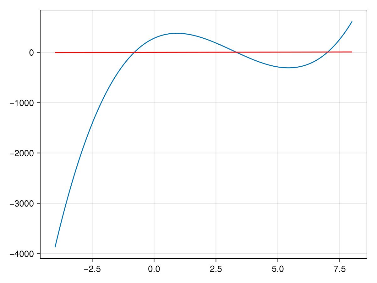
Solving an equation is a very important part of mathematics and other scientific fields. However, finding general solutions to equations is not very easy. Consider a cubic equation like \(x^{3}-10x^{2}+24x-17\text{.}\) In the spirit of (but not very simple) the quadratic formula, there is a cubic formula. Much of the wikipedia page spends time solving the cubic with all possibilities. In short, it’s not very easy.
This cubic actually factors, but finding those factors is quite difficult to do in general. We then look at using Newton’s method to solve this. Note the plot below:
We are going to go through building a function to do this. First, let’s consider the template of the function, which will have an arguments f, df and x0. Thus a good template is
You will need to do the two steps above many times so you will need a loop. Since you don’t know how many times you will need to run through the loop use a while loop and your condition should be that the two steps x0 and x1 are apart from each other.
Checking if two floating-point numbers are equal are generally not a good idea, because they have to be equal to all bits, so instead we will run the while loop while the difference in the numbers x0 and x1 are larger than some default (like \(10^{-6}\)).
function newton(f::Function, df::Function, x0::Number)
  x1 = x0 - f(x0)/df(x0)
  while abs(x1-x0) > 1e-6 # while the two numbers are larger than 10^(-6)
    x0 = x1
    x1 = x0 - f(x0)/df(x0)
  end
  x1
end
Just to simplify this, we will define dx as -f(x0)/df(x0), which is the distance between successive x values, so we’ll use this to determine when to stop the loop:
function newton(f::Function, df::Function, x0::Number)
  local dx = f(x0)/df(x0)
  local x1 = x0 - dx
  while abs(dx) > 1e-6
    dx = f(x1)/df(x1)
    x1 -= dx
  end
  x1
end
First, we need to define dx first to determine if we need to go into the loop. We just set it to some value to get it started. We have also used the operator -=. Line 6 above or x1 -= dx is shorthand for x1 = x1 - dx
function newton(f::Function, df::Function, x0::Number)
  local dx = f(x0)/df(x0)
  x0 -= dx
  while abs(dx) > 1e-6
    dx = f(x0)/df(x0)
    x0 -= dx
  end
  x0
end
We have changed a few things. First, note that we decided to reuse the variable x0 to keep track of the current root instead of introduce a new variable. In some languages, this would not be a good idea in that using arguments will change those outside the scope of the function. However, in Julia is not the case and in Section 11.7, we go into details about how function arguments are passed.
And note that we have used x0 -= dx which is a shortcut for x0 = x0 - dx. One note from a programming point of view is that we have repeated code (lines 2 and 3 are the same as lines 5 and 6). Unfortunately this is needed because we need to know dx before entering the loop and then also need to update it within the loop. We will shorten this a bit later.
If you have used Computational Algebra Systems like Maple or Mathematica, you know that computers have the ability to differentiate. Julia does not have this capability built-in, although it has some capability of doing some of the feature set of these programs. There is a system called automatic differentiation that will compute the exact derivative to a function at a given point. That is, if you have a function \(f(x)\) and a number \(a\text{,}\) it will give you \(f'(a)\text{.}\) The package is called ForwardDiff and you may need to add it and then
which returns 0.2658898634234979 and if you are careful with the derivative (or have access to a Computer Algebra System), see if your answer is correct.
function newton(f::Function, x0::Number)
  local dx = f(x0)/ForwardDiff.derivative(f, x0)
  x0 -= dx
  while abs(dx) < 1e-6
    dx = f(x0)/ForwardDiff.derivative(f, x0)
    x0 -= dx
  end
  x0
end
Notice that we no longer need the derivative for this function, since the ForwardDiff package will compute it for us, thus the function signature has changed.
Find the intersection point of the functions \(y=x\) and \(y=\sin x\text{.}\) Hint set the two equations equal and use algebra to write it as a function \(g(x)\) which is equal to 0.
Subsection10.4.4Adding an extra stopping condition
One problem that can arise is if you call newton on a function that does not have a root. For example, consider \(f(x)=x^2+1\text{,}\) which is always positive. If you run
To prevent this, we need to add a stopping condition if this occurs. One way to do this is to add a counter include in the while loop that the number of steps is small. Here’s a possible update to Newton’s method:
Now, this still isn’t perfect because when we run it, we only get a single number out. In this case, the value is not a root, but how do you know? We will see in Chapter 12 how to develop a new type which stores information about the root and if a solution was reached.
Subsection10.4.5Newton’s method: Alternative Formulation
Looking at the code in Listing 10.7, recall that we used a while loop to perform this because we don’t know the number of steps it takes. However, we do have a maximum number of steps and in a case like this a for loop might be nicer.
function newton(f::Function, x0::Number)
  for _ = 1:10
    dx = f(x0)/ForwardDiff.derivative(f, x0)
    x0 -= dx
    abs(dx) < 1e-6 && return x0
  end
  x0
end
There are a number of things to notice here. First, we have started with a for loop. In Listing 10.7 we needed to define some variables before entering the while loop, so the above code is shorter. Also notice that since we don’t really need the index of the loop we have used the convention of the _ variable. Lines 3 and 4 are identical to above to compute dx, which is the step of newton’s method and updating x0. Lastly, we want to break out of the loop (and the function) and return the current value of x0 if the step size is small enough. We use the shorthand if for this on line 5.
After redefining newton’s method with that in Listing 10.8, ensure that it is still working by finding all three roots of \(f(x) = 15x^3 - 143x^2+266x+280\text{.}\)
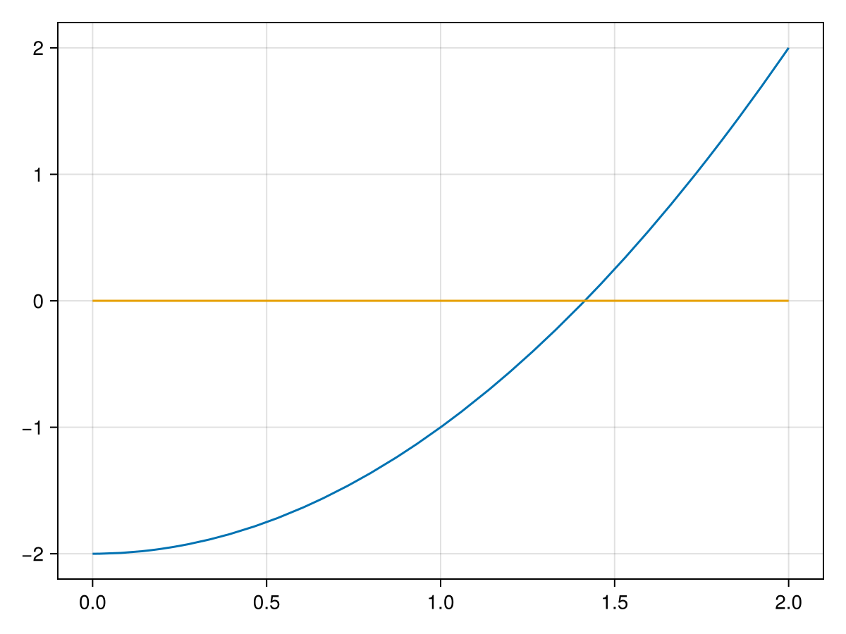
In Subsection 5.4.1, we saw the bisection method and just presented it as an example of using a while loop. We return to this to further explain the method. If we have a function like \(f(x) = x^2-2\) and seek to find a root of this 1
Yes, I realize this is an example where we know the answer using algebra, but go with it.
and note that we are seeking where the curve crosses the \(x\)-axis. The bisection method requires that we start with an interval that contains the root. In this case, we will use \([a_0,b_0]=[1,2]\text{.}\) We know that there is a root of this from the intermediate value theorem which states that a continuous function takes on all values between \(f(a)\) and \(f(b)\text{,}\) where \(a\) and \(b\) are the endpoints of the interval. Since we are seeking a value \(x^{\star}\) where \(f(x^{\star})=0\text{,}\) the endpoints must have opposite signs which can be tested by multiplying the values and testing for a negative number or \(f(a)f(b) < 0\text{.}\)
Let a and b be an interval \([a,b]\) such that f(a)*f(b) < 0 . The following uses the bisection method to find a root to within ϵ of the true value \(x^{\star}\text{.}\)
function bisection(f::Function, a::Real, b::Real)
  local c
  while b-a > 1e-6
    c = 0.5*(a+b)  # find the midpoint
    # test if f(a) and f(c) have opposite signs to determine the new interval
    (a,b) = f(a)*f(c) < 0 ? (a,c) : (c,b)
  end
  c
end
where we have hard coded ϵ to be 1e-6. Note also that we have used a tuple to store the interval and have updated the entire interval instead of just one endpoint as the algorithm above states. This is mainly for code clarity. Also, we will update this code to handle other values of ϵ in Chapter 11. Also in that chapter we will test to ensure that the original interval contains the root.
You may also question why we have line 2, which doesn’t see to do anything. This is crucial (try commenting out the code and rerunning--you will get an error). This is due to the scope of the variable c, which will be explained in more detail in Section 11.6.
Running the code with x0 = bisect(x -> x^2-2, 1, 2) returns 1.4142141342163086 and absErr(x0, sqrt(2)) returns 5.718432134482754e-7 showing that in fact the error is with \(10^{-6}\text{.}\)
function bisection(f::Function, a::Real, b::Real)
  while true
    c = 0.5*(a+b)  # find the midpoint
    (a,b) = f(a)*f(c) < 0 ? (a,c) : (c,b)
    (b-a) < 1e-6 && return c
  end
end
where we have used the while true loop, which can be dangerous since it may result in an infinite loop, but line 5 is the way to break out of the loop and the function.