Chapter 37 Linear Regression
One common task when having a dataset is to build a model of the data and a common model is a linear one. Consider the
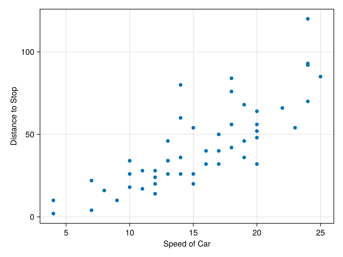
cars dataset in the RDatasets package. This dataset is a simple two column set with the speed a car is travelling and the distance it takes to reach a full stop. A scatter plot of the data is:
cars=RDatasets.dataset("datasets","cars")
fig = Figure()
ax = Axis(fig[1,1], xlabel="Speed of Car", ylabel = "Distance to Stop")
scatter!(ax, cars.Speed, cars.Dist)
fig
The plot reveals that the faster the car is traveling, the longer it takes to stop. This probably isn’t a surprise, but perhaps we’d like to know the relationship between then. That is, can we predict the stopping distance if we know the speed of the car. The simplest model to use for this is a linear one.
Section 37.1 Basics of Linear Regression
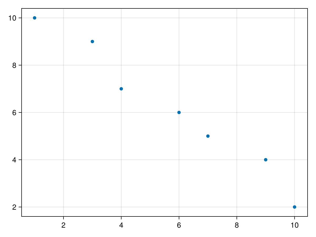
Before finding the linear model for the above example, let’s look at a simpler dataset. Consider
data = DataFrame(x=[1,3,4,6,7,9, 10], y = [10, 9, 7, 6, 5, 4, 2])
and has the following scatter plot:
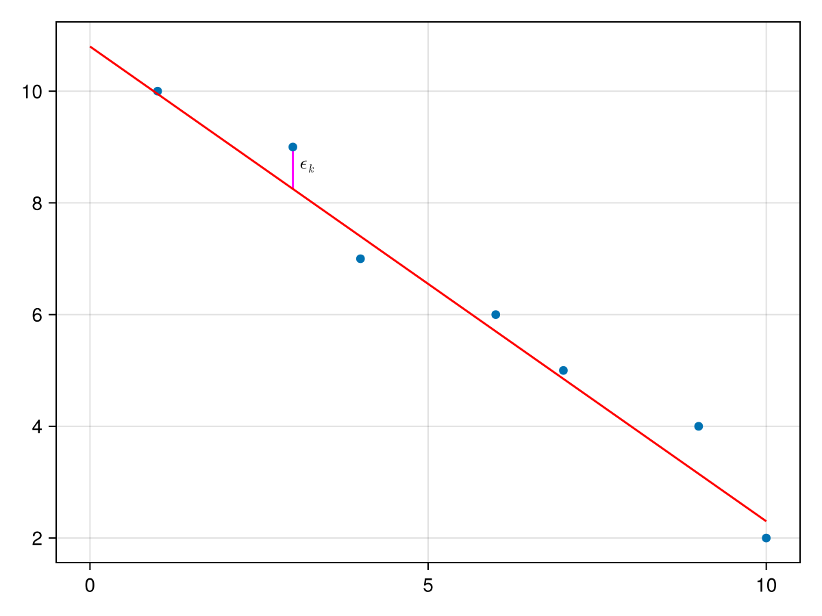
We seek a line of the form \(y=ax+b\) which we plot below and for each data value, we define \(\epsilon_k = y_k - (a x_k+b)\text{,}\) which is the vertical signed distance between the line and the data as shown below:
We then find the total square distance of all of the errors as
\begin{equation}
S(a,b) = \sum_{k=1}^n (y_k - (ax_k+b))^2\tag{37.1}
\end{equation}
which is explicitly stated as a function of \(a\) and \(b\text{,}\) the slope and \(y\)-intercept of the line. The best fine line then is the line that minimizes this function. To find the values of \(a\) and \(b\text{,}\) there are many techniques to accomplish this. We find the derivatives \(\partial S/\partial a\) and \(\partial S/\partial b\text{,}\)
\begin{align}
\frac{\partial S}{\partial a}\amp = 2 \sum_{k=1}^n(y_k -(ax_k+b))(-x_k) \notag\\
\amp = -2 \sum_{k=1}^n x_k y_k + 2 a \sum_{k=1}^n x_k^2 + 2 b \sum_{k=1}^n x_k \notag\\
\amp = -2 S_{xy} + 2 a S_{xx} + 2b S_x \tag{37.2}\\
\frac{\partial S}{\partial b} \amp = 2 \sum_{k=1}^n(y_k - (ax_k+b))(-1) \notag\\
\amp = - 2 \sum_{k=1}^n y_k + 2a \sum_{k=1}^n x_k +2b \sum_{k=1}^n 1 \notag\\
\amp = - 2 S_y + 2a S_x + 2nb \tag{37.3}
\end{align}
where
\begin{align}
S_x \amp = \sum x_i, \amp \quad S_y \amp= \sum y_i, \amp S_{xx} \amp = \sum x_i^2, \amp \quad S_{xy} \amp = \sum x_i y_i,\amp \quad S_{yy} \amp = \sum y_i^2 \tag{37.4}
\end{align}
\begin{align}
a \amp = \frac{n S_{xy} -S_x S_y }{n S_{xx} - S_x^2}\amp b \amp = \frac{1}{n} \left( S_y - a S_x \right) \tag{37.5}
\end{align}
Sx = sum(data.x)
Sy = sum(data.y)
Sxx = sum(x -> x^2, data.x)
Sxy = sum(data.x .* data.y)
Syy = sum(y -> y^2, data.y)
where in the case of the 3rd and 5th line above, we have used the option for
sum that takes a function and applies the function to the array element and then sums. With these given terms, we can find \(a\) and \(b\) with
a = (length(data.x)*Sxy - Sx*Sy)/(length(data.x)*Sxx-Sx^2)
b = (Sy-a*Sx)/length(data.x)
a,b
and this returns
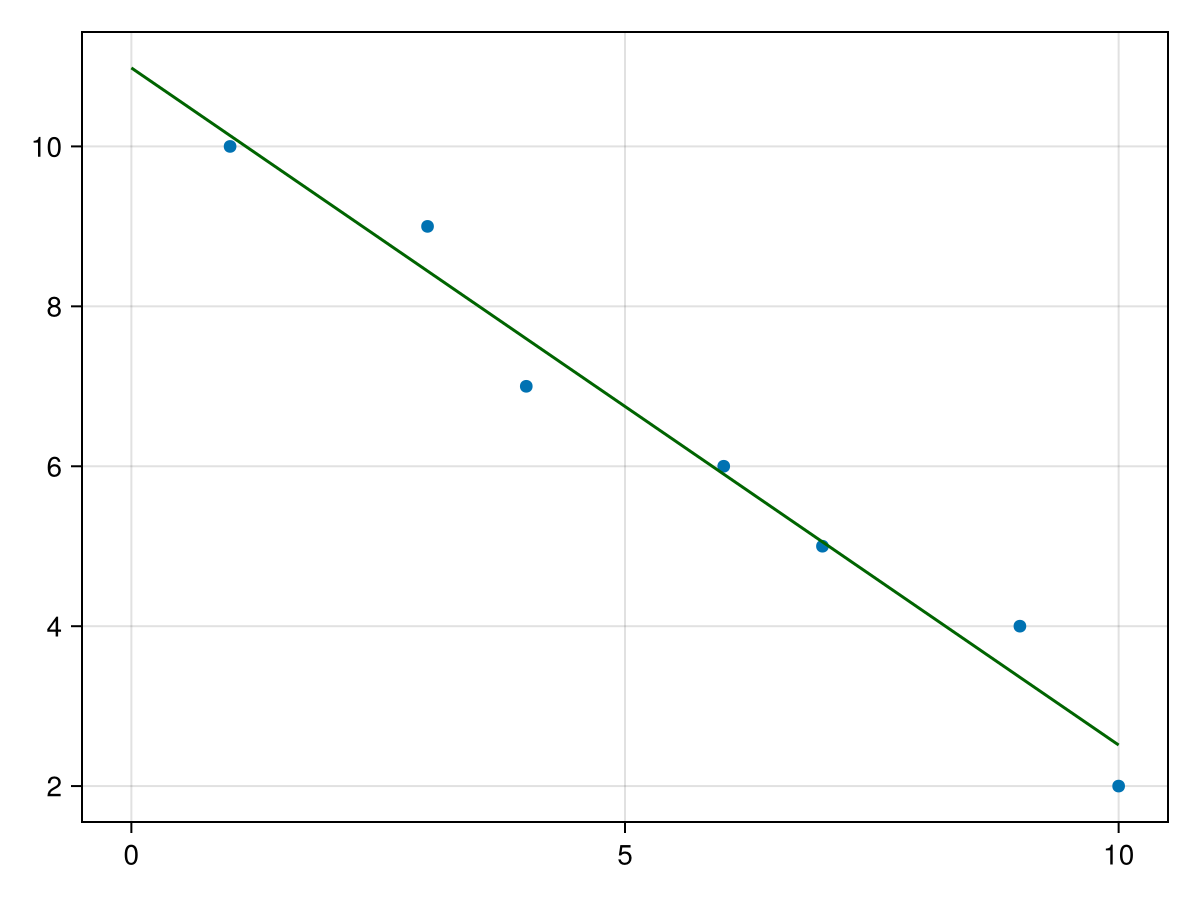
(-0.8468468468468469, 10.981981981981983) for a and b respectivley. The best fit line is then \(y=10.98198 - 0.8468 x\text{.}\) We can use this to plot the data and the best-fit line as follows:
fig, ax = scatter(data.x,data.y)
lines!(ax, 0..10, x -> a*x+b, color = :darkgreen)
fig
which produces the following plot:
This looks good visually, but how do we know it is a good fit. There are a number of parameters that we can use to calculate the fit and the next sections goes briefly into this.
Section 37.2 Measures of Regression
As we saw in the previous section, visually the fit of the example above looks good, but it would be nice to have a measure (numerical value) of the fit. We will explore this in this section.
First, we introduce the notion of the residuals for a regression, in short this is
\begin{equation*}
\epsilon_i = y_i - (ax_i+b)
\end{equation*}
where \(a\) and \(b\) are the best fit slope and intercept. In terms of a plot, each \(\epsilon_i\) is the vertical distance between a datapoint and the regression line.
There are two important measures here, the sum of squares regression or
\begin{equation*}
\text{SSR} = \sum \epsilon_i^2
\end{equation*}
Again, as we mentioned in the previous section, the goal of regression is to find the regression coefficients (in this case the slope and intercept) that minimize this value.
For the example above, we can find the SSR in Julia with
SSR = sum([(data.y[i] - a*data.x[i]-b)^2 for i=1:nrow(data) ])
and this returns
1.3693693693693667. The sum of squares error or
\begin{equation*}
\text{SSE} = \sum (y_i - \bar{y})^2
\end{equation*}
The SSE can be written as:
\begin{equation*}
\text{SSE} = S_{yy} - \frac{1}{n} S_y^2
\end{equation*}
is a sum of squares of the vertical distance between the \(y\)-value of each datapoint and the mean. Using the example above, we have already calculated \(S_{yy}\) and \(S_y\) so
SSE = Syy -Sy^2/nrow(data)
resulting in
46.85714285714283. A nice measure of the fit of the regression line is by using the following:
\begin{equation*}
r^2 = 1 - \frac{\text{SSR}}{\text{SSE}}
\end{equation*}
The value of \(r^2\) satisfies \(0 \leq r^2 \leq 1\) and a proof is left to the reader. The closer the value is to 1, the better the fit and in fact when \(r^2=1\text{,}\) then the data perfects lies on a line.
For the example above
rsq = 1-SSR/SSE
resulting in
0.970775653702483, which is a good fit, where 97% of the variability in the data is explained with the linear model.
Section 37.3 A Matrix Approach to Linear Regression
The above formulas for linear regression works only for a best-fit line through a set of points \((x_k, y_k)\text{.}\) If we want to either fit other functions, one needs to find another way. A more general way is to define
\begin{align*}
X \amp = \begin{bmatrix} 1 \amp x_1 \\ 1 \amp x_2 \\ \vdots \\ 1 \amp x_n \end{bmatrix} \amp \amp \vec{y} = \begin{bmatrix} y_1 \\ y_2 \\ \vdots \\ y_n \end{bmatrix} \amp \vec{c} \amp = \begin{bmatrix} a \\ b \end{bmatrix}
\end{align*}
\begin{equation}
S(a,b) = (X \vec{c} - \vec{y})^T (X \vec{c}-\vec{y})\tag{37.6}
\end{equation}
and differentiating with \(\partial_{\vec{x}} [(\vec{F}(\vec{x}))^{\intercal} \vec{F}(\vec{x})] = 2 \vec{F}(\vec{x})^{\intercal} \vec{F}(\vec{x})\) leads to
\begin{align*}
\frac{\partial S}{\partial \vec{c}} \amp = 2 X^{\intercal} (X \vec{c} - \vec{y})\\
\amp = 2 X^{\intercal} X \vec{c} - 2 X^{\intercal} \vec{y}
\end{align*}
\begin{equation*}
\vec{c} = (X^{\intercal} X)^{-1} X^{\intercal} \vec{y}
\end{equation*}
We now apply this to the above example. First, we will create the
X matrix with the following:
X = [data.x[i]^k for i=1:nrow(data), k=0:1]
which generates the matrix with ones in the first column and
data.x in the second. And then
c = inv(X'*X)*X'*data.y
where
X' is the way to find the transpose of X in julia. The result is the vector [ 10.982, -0.8468], which is the vector of \(y\)-intercept and slope. So the best-fit line for this is \(y=-0.8468x+10.982\text{.}\)
Section 37.4 Fitting Other Functions to Data
As mentioned above, we may want to fit other functions to a set of data. For example, if we want to fit the following data to a quadratic.
Subsection 37.4.1 Fitting a Quadratic to Data
data2 = DataFrame(x =-4:4, y = [15, 10, 5, 2, 1, 0, 3,8, 17])
which has the following scatter plot
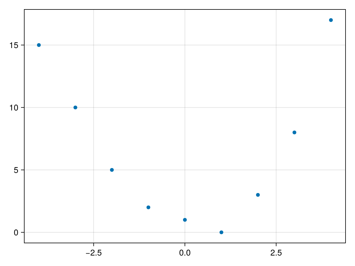
It appears that the data might fit a quadratic curve of the form \(q(x) = ax^2+bx+c\text{.}\) Similar to above, we desire to find the constants \(a, b\) and \(c\) such that
\begin{equation*}
S(a,b,c) = \sum_{k=1}^n (y_k - (a_2 x_k^2 + a_1 x_k + a_0))^2
\end{equation*}
is minimized. We will write in the same way using matrix as
\begin{equation}
S(a,b,c) = (X \vec{c})^{\intercal} X \vec{c}\tag{37.7}
\end{equation}
with
\begin{align*}
X \amp = \begin{bmatrix} 1 \amp x_1 \amp x_1^2 \\ 1 \amp x_2 \amp x_2^2 \\ \vdots \\ 1 \amp x_n \amp x_n^2 \end{bmatrix} \amp \amp \vec{y} = \begin{bmatrix} y_1 \\ y_2 \\ \vdots \\ y_n \end{bmatrix} \amp \vec{c} \amp \begin{bmatrix} a_0 \\ a_1 \\ a_2 \end{bmatrix}
\end{align*}
and since (37.7) has the same form as (37.6), to find the values \(\vec{c}\) that minimizes (37.7) is the same or
\begin{equation*}
\vec{c} = (X^{\intercal} X)^{-1} X \vec{y}
\end{equation*}
For the example at the top of this section, we define
X = [data2.x[k]^i for k=1:nrow(data), i=0:2]
Then we can find the coefficients with
c = inv(X'*X)*X'*data2.y
The result of this is
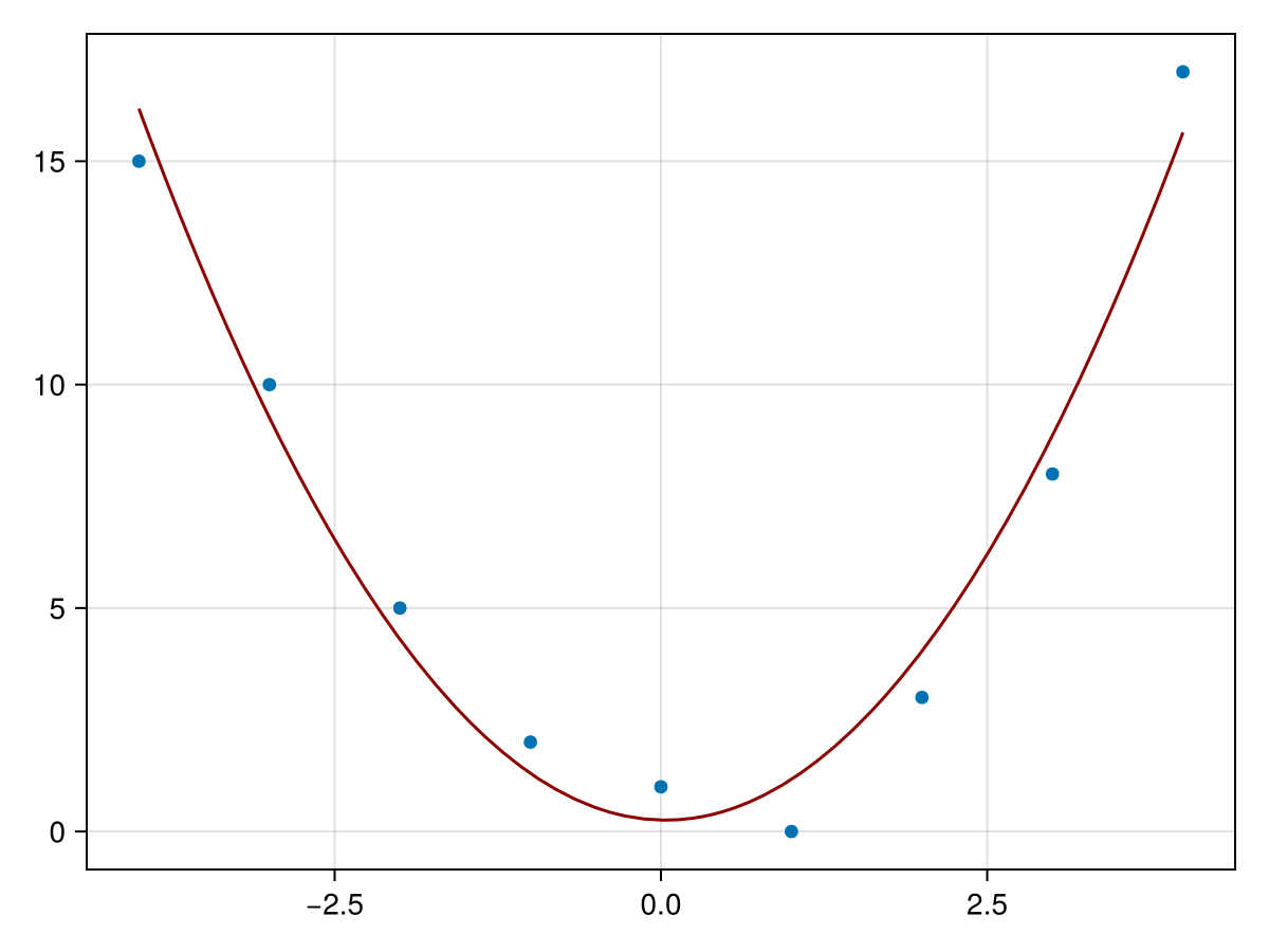
[0.255, -0.0666, 0.978]. Therefore the best-fit quadratic is
\begin{equation*}
q(x) = 0.978 x^2 -0.0666 x + 0.255
\end{equation*}
A plot of the data and the function is given by
Subsection 37.4.2 Multilinear Regression
Another common function used to fit to data is that of a linear function in higher dimensions. As an example, consider the following dataset:
data3 = DataFrame(
  x = [1, 1, 2, 3, 3, 4, 5, 5, 6, 2, 4, 8],
  y = [1, 6, 8, 2, 2, 3, 7, 3, 1, 4, 9, 6],
  z = [14, 7, 4, 14, 13, 12, 7,  13, 16, 11, 4, 10])
which has the plot
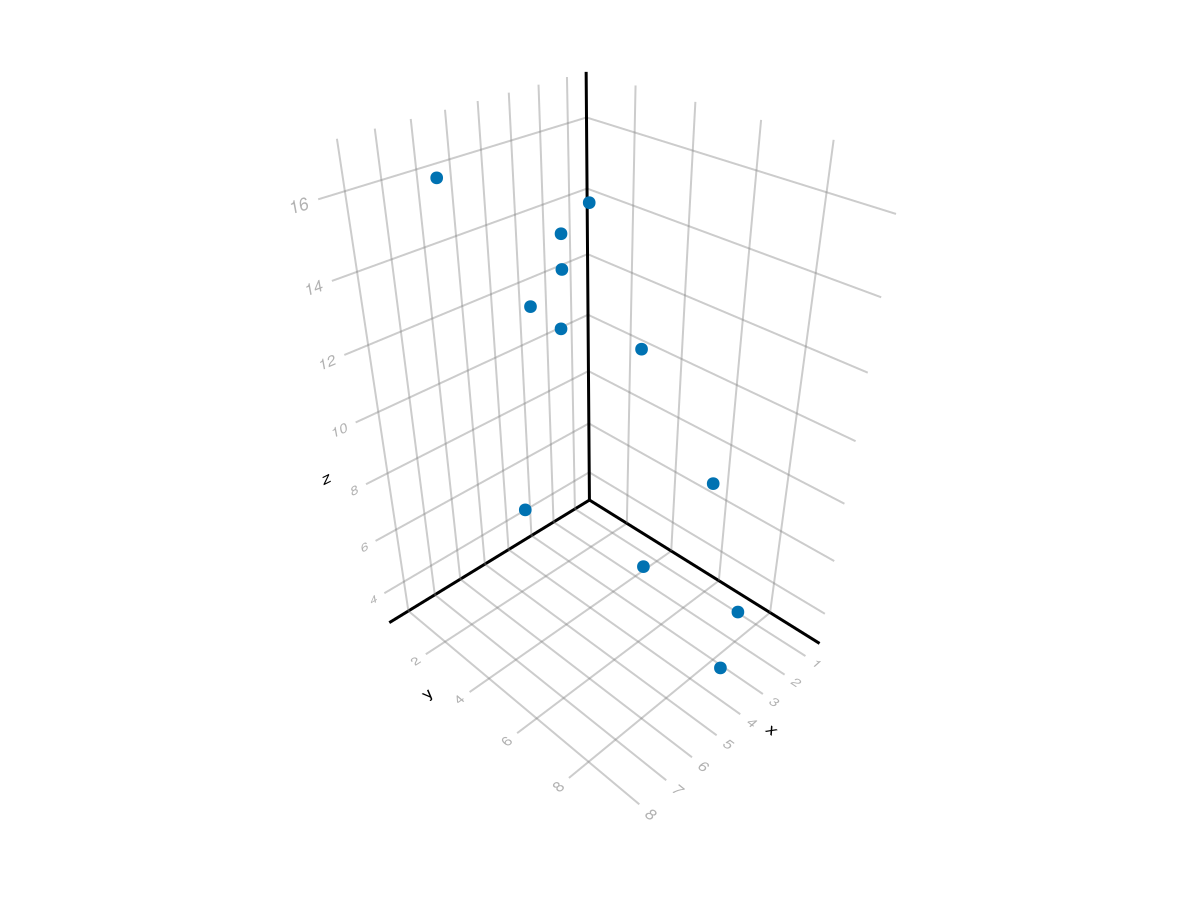
Although this is difficult to tell, these points roughly fall on a plane, so we can fit a plane of the form \(z = a_0 + a_1 x + a_2 y\) to the data. This can be done with the matrix form by setting the first column to 1, the second column to \(x\) and the third to \(y\) or
X = ones(Int,size(data3,1),3)
X[:,2] = data3.x
X[:,3] = data3.y
X
and again using the same formula as above to find the best-fit coefficients:
c = inv(X'*X)*X'*data3.z
resulting in
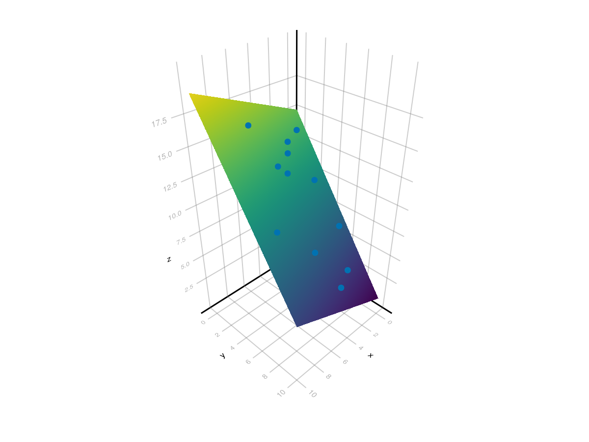
[15.13, 0.4085, -1.433] which is the plane \(z = 15.13+0.4085x-1.433y\text{.}\) A plot of the plane and the points is found with:
xpts = ypts = LinRange(0,10,100)
fig, ax = surface(xpts, ypts, [c[1].+c[2].*x .+ c[3] .* y for x in xpts, y in ypts])
scatter!(ax, data3.x, data3.y, data3.z)
fig
resulting in the following plot. Note: to get the interactive version of this plot, use
GLMakie and set Makie.inline!(false) to ensure a separate window which allows the plot to rotate interactively.
Section 37.5 Linear Regression with GLM package
There is a robust packge for regression called
GLM short for Generalized Linear Models, which allows many different kinds of regression performed on a dataset. Make sure that you have added this package and loaded it with using GLM.
To start with a simple model, we can produce a best fit line with the formula
y ~ x, meaning that we want y, which is a column in our data Dataframe as the dependent variable to be linear in x the column that will be the independent variable. After creating a formula with the @formula macro, we fit the data with the lm short for linear model method as in:
fm = @formula(y ~ x)
model = lm(fm, data)
The result is
y ~ 1 + x

Coefficients:
──────────────────────────────────────────────────────────────────────────
                 Coef.  Std. Error       t  Pr(>|t|)  Lower 95%  Upper 95%
──────────────────────────────────────────────────────────────────────────
(Intercept)  10.982      0.4244      25.88    <1e-05    9.89103  12.0729
x            -0.846847   0.0657102  -12.89    <1e-04   -1.01576  -0.677933
──────────────────────────────────────────────────────────────────────────
There are a number of things to note here:
-
The top line is the formula
y ~ 1 + xwhich is the same asy ~ x. The1denotes that you want to include a constant term in your formula. Note: you can doy ~ 0 + xto force no constant term. -
The cofficients table has information about all of the coefficients, in this case 2, the constant term and the coefficient of the
xterm. The first column is which coefficient and the second is the best-fit value of this coefficient. Notice that this is the same as we found above using the derived formulas. -
The remainder of the table indicate statistics to determine the significance of each of the coefficients. The
Pr(> |t|)is the \(p\)-value for each of the coefficients differs from 0. In this case, each are highly significant due to the small values. The last two columns give a confidence interval. To 95% confidence, each coefficient is between the last two columns.
Additionally, we can determine the overall fit of the model with an \(r^2\) value. This is accomplished with
r2(model) which returns 0.970775653702483. A standard interpretation of this is that the linear model explains 97% of the variation in the data. This represents a very good linear fit.
Subsection 37.5.1 Finding the best-fit quadratic with GLM
You may be surprised to learn that the quadratic fit is actually a linear model. But wait, you say, I learned in Precaclulus that a quadratic function is not linear and that is true. But recall that the linearity is in the unknown coefficents and those are linear.
To find the best-fit quadratic using GLM, we first build the quadratic formula with
fm2 = @formula y ~ 1 + x + x^2
and although you don’t need to include the 1, I would recommend putting it in for any non linear function. This will correspond to fitting to a function of the form \(y = a_0 + a_1 x + a_2 x^2\text{.}\)
To find the coefficients, we’ll use
model2 = lm(fm2, data2)
which returns
y ~ 1 + x + :(x ^ 2)

Coefficients:
──────────────────────────────────────────────────────────────────────────
                  Coef.  Std. Error      t  Pr(>|t|)  Lower 95%  Upper 95%
──────────────────────────────────────────────────────────────────────────
(Intercept)   0.255411     0.600744   0.43    0.6855  -1.21456    1.72538
x            -0.0666667    0.153459  -0.43    0.6792  -0.442168   0.308835
x ^ 2         0.978355     0.067732  14.44    <1e-05   0.812621   1.14409
──────────────────────────────────────────────────────────────────────────
and we’ll find the \(r^2\) value with
r2(model2)
which returns
0.972071266946816, which is surprisingly close to the previous example, but just shows that the overall model is a good fit. However, looking at the table above, only the \(x^2\) term is significantly different from 0, with a \(p\)-value much less that 0.05, the standard cutoff level.
Subsection 37.5.2 Multilinear Regression with GLM
The example using the dataset
data above was fit with two predictor variables, x and y. To build the formula and then the model is done with
fm3 = @formula z ~ x + y
model3 = lm(fm3, data3)
and this returns
z ~ 1 + x + y

Coefficients:
──────────────────────────────────────────────────────────────────────────
                 Coef.  Std. Error       t  Pr(>|t|)  Lower 95%  Upper 95%
──────────────────────────────────────────────────────────────────────────
(Intercept)  15.134      0.32197     47.00    <1e-11  14.4056    15.8623
x             0.408533   0.0623703    6.55    0.0001   0.267442   0.549625
y            -1.4343     0.0472865  -30.33    <1e-09  -1.54126   -1.32733
──────────────────────────────────────────────────────────────────────────
and finding the \(r^2\) value with
f2(model3) returns 0.9905202860004992, a very good fit and examining the Pr(>|t|) column all of the coefficients are significant.
