“A round table has 7 chairs around it. Mary and her friend Alisha and 5 other people are given seats at the table in a random manner. What is the probability that Mary and Alisha sit next to each other?”
Although it is an good skill to solve problems like these using counting techniques, we examine some ways to use simulation to find the solution in this chapter.
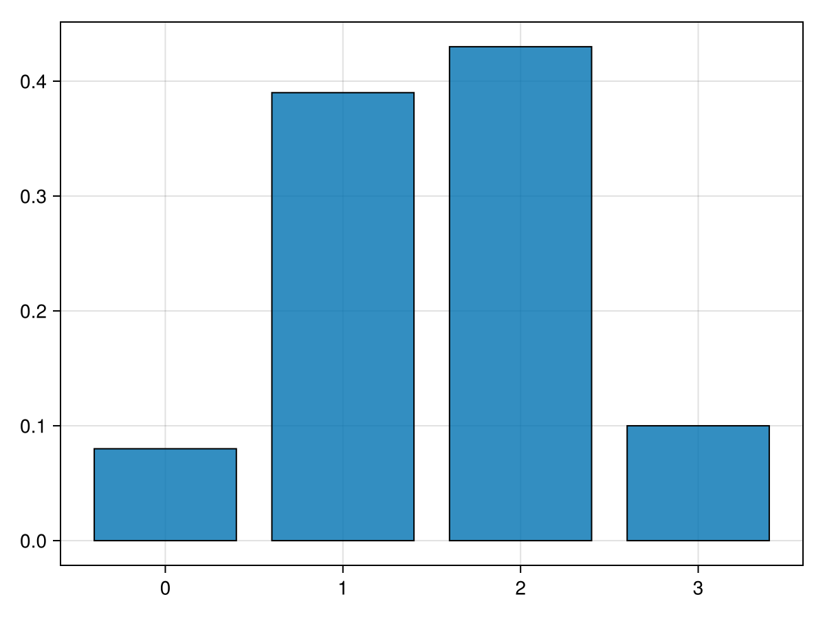
Another simple example is to flip multiple coins and generally count the number of heads or tails seen. Consider flipping 3-coins--perhaps a penny, nickel and dime--and counting the number of heads. We then do that 3-coin flip a larger number of times.
Each row contains the coin flips. Each 1 represents a head and 0 is a tail. If we are interested in the sum of the number of heads, we can do this with the mapslices functions seen in Chapter 6.
The first few elements of the array is [2; 1; 1; 2; 2; 1; 1; 0 ...]. We would like a plot of this, however need to do a bit of work first. The hope is that for each number of heads 0, 1, 2 and 3, we create a bar plot with the number of heads for each or the fraction of heads. Although we have the tools to do this, since this is a common thing to do in statistics, there is a function in the StatsBase package.
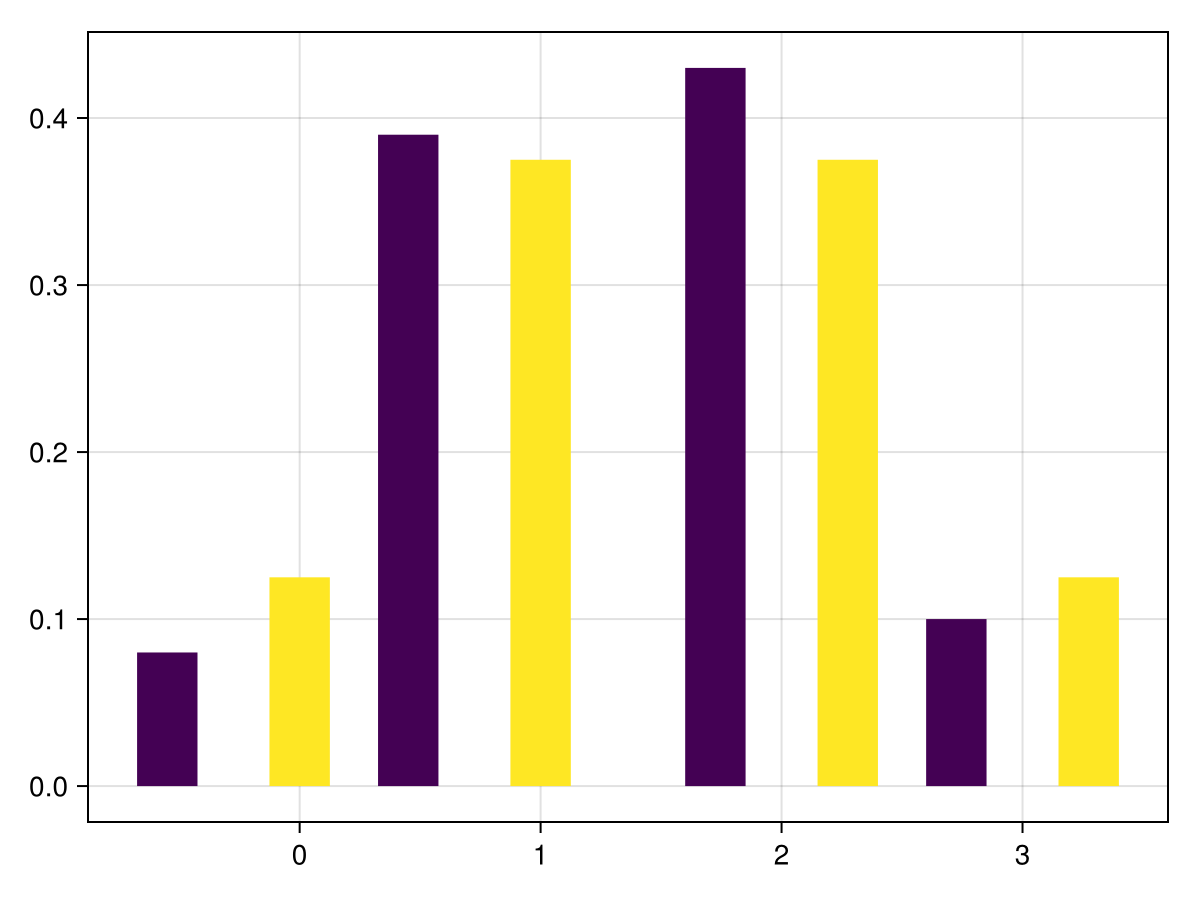
which generates an approximate probability distribution for flipping 3 coins and s umming the number of heads. And to compare the simulation with the probability density function that we found in Chapter 18, we will plot a side-by-side comparison of the two with the following. Note that the function groupedbar is part of the StatsPlots package:
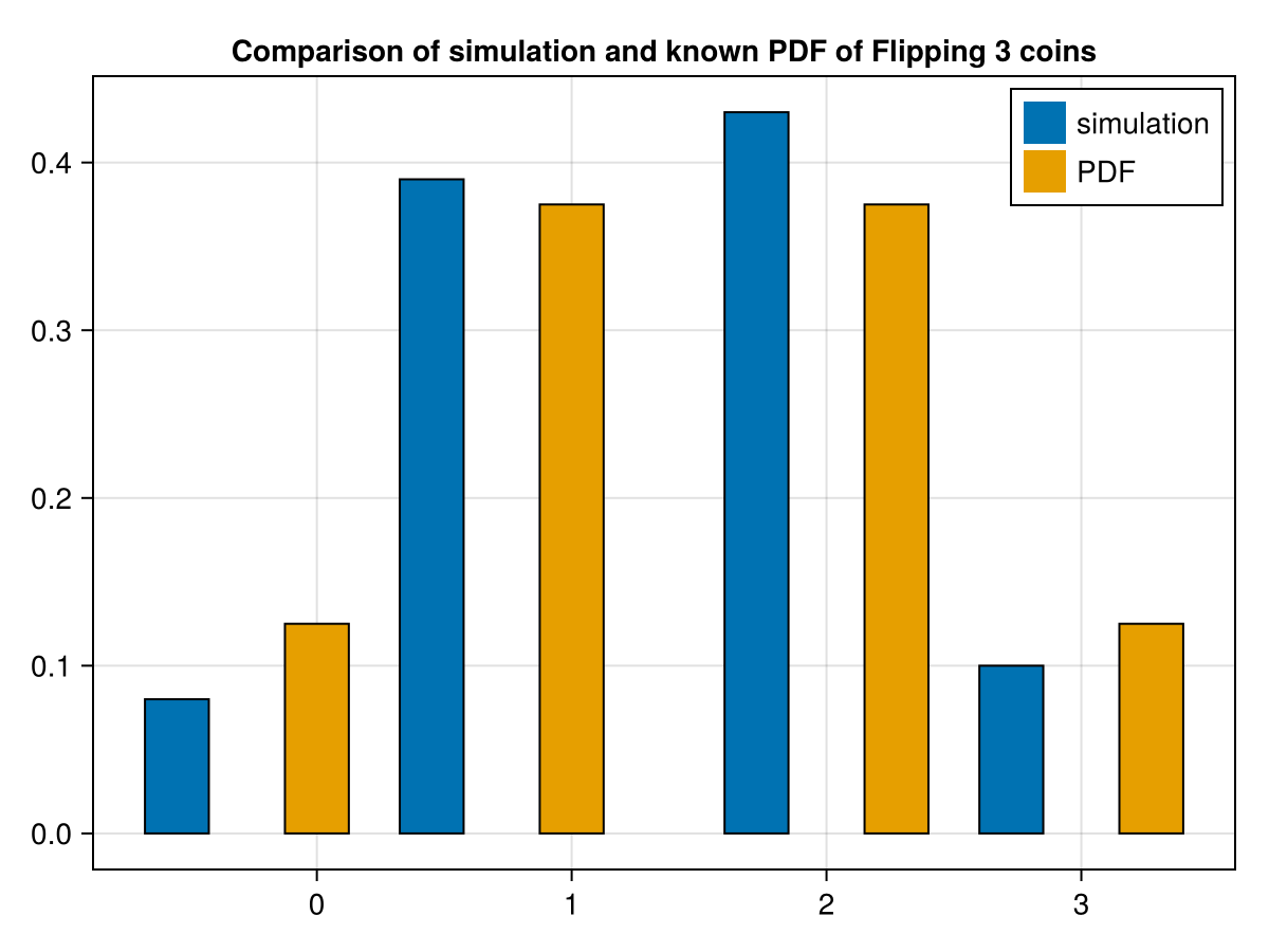
This is not the best looking plot and would like to include a legend. Here’s a little cleaned up version of this and then will explain all of the arguements and attributes.
This is reasonably complicated and for a grouped bar plot and there are many ways to do this using the barplot method and we go into a lot of details in Chapter 32. To use this with other data, you should be able to update the first 3 lines of this code.
A relatively-simple example is that of rolling dice. As we saw in Chapter 18, if we have a fair, six-sided die, the the probability of any of the numbers coming up is 1/6. We can simulate that using random numbers in the following way:
The principal of the Law of Large Numbers is that as a experiment is repeated, as the number of times increases, the distribution of results tends toward the underlying distribution. If we determine if this is true, as the number of time we roll a die increases, the probability of any one number appearing gets closer to 1/6. For example, to test this, try
p = count(a->a==3,rand(1:6,1_000))
and then evaluating p/1_000 results in 0.190, which is reasonably close to 1/6.
Trying increasing the number of random numbers used in the above example. You should notice that as that number gets larger, the resulting probability gets closer to 1/6.
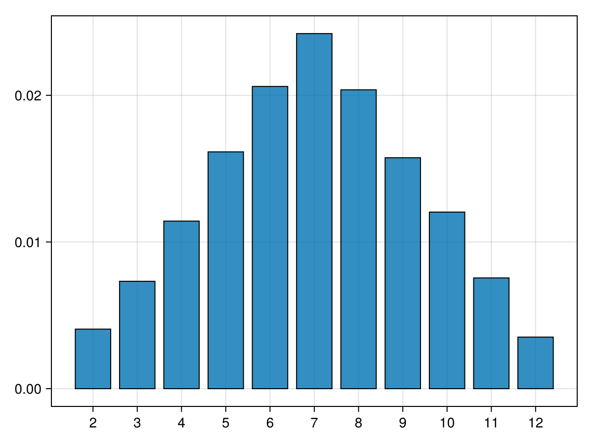
How do we handle the rolling of two dice? We will do this in a similar manner to flipping 3 coins above. First, we’ll start with an array with each row having 2 dice. This would be a simulation of rolling 10,000 pairs of dice.
which creates a matrix of size of 10,000 by 2 of random numbers between 1 and 6. Each row represents a pair of dice and the sum of the dice is just the sum of each row which we can get from
which sums along the rows. This is 10,000 rolls of 2 dice with the sum recorded. First, to get an idea of the distribution of the dice sums, let’s plot the distribution of the values:
where we use generic names for the other 5 people. 2
Although variable name usually don’t matter what they are called, names cannot be used. There are many function and variable names that cannot be used. This is one example.
We will take random permutations of this array below and the determine if Alisha and Mary are next to each other.
Before we find a random permutation, let’s write a function that takes an array of names and returns true if they are next to each other and false if not.
function nextToEachOther(names::Vector{String})
  a = findfirst(name -> name=="Alisha",names)
  m = findfirst(name -> name=="Mary",names)
  abs(a-m) == 1 || abs(a-m) == length(names)-1
end
where the findfirst function returns the index of the array where the function is true (that is where the two friends are sitting). To test this:
returns ["p3" "Alisha" "Mary" "p5" "p2" "p4" "p1"], then we can test if they are sitting next to each other. The follow repeats this a large number of times:
function numTimes(trials::Integer)
  s = 0  # keeps track of how many times they sit next to each other
  for i=1:trials
    if nextToEachOther(shuffle(table_names))
      s += 1
    end
  end
  s/trials
end
and then the fraction of times is found with numTimes(10_000) resulting in 0.3303.
The true value of the probability can be found in the following way. Mary sits in one of the seven chairs. Alisha has a equal chance of sitting in one of the remaining 6 chairs. Two of the chairs are next two Mary, so the probability is 2/6 or 1/3. The result we see above is close to this value.
Section19.5Calculating \(\pi\) using pseudo random numbers
You probably know the first handful of digits of \(\pi\) and recall that probably the first place that you saw this was with circles. But how do we know what the digits of \(\pi\) actually are. There are a number of ways to find the digits of \(\pi\) and in fact, Chapter 48 presents some interesting ways of calculating it.
In the 18th Century, Georges-Louis Leclerc, Comte de Buffon considered the following problem. On a floor (or table), draw lines that are parallel and \(t\) units apart. Toss needles of length \(\ell\) onto the floor and count the number that cross one of the lines. The following diagram is helpful:
So theoretically, one could sit and toss needles onto a floor to determine the value of \(\pi\) by counting the number that cross the lines and those that don’t. This would be tedious and possibly prone to error as the number of needles rises.
The Buffon Needle experiment is fascinating in many ways but there is a much easier way to generate results in a computer simulation. This is called the Circle in the Square approach.
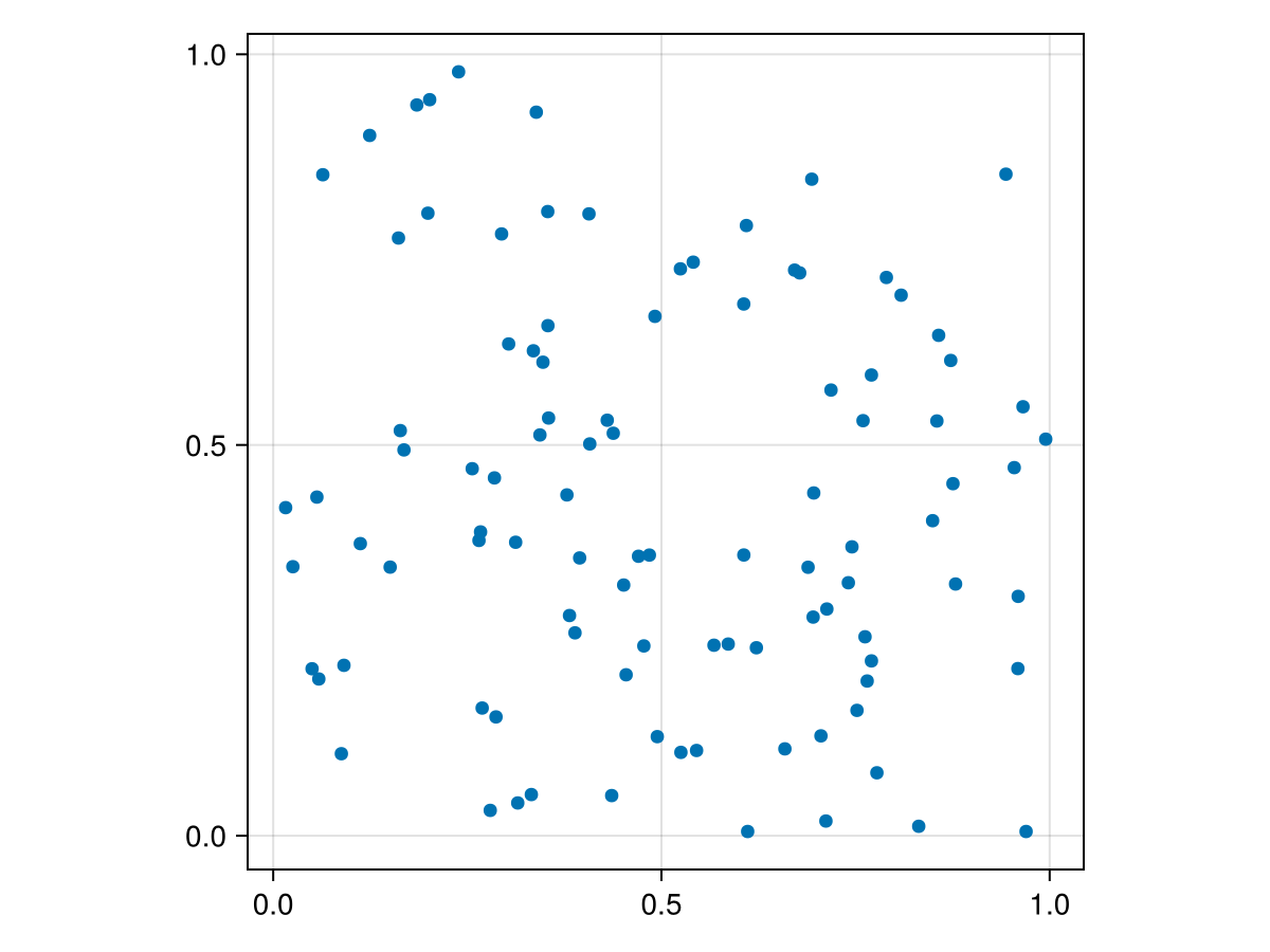
Consider a square given by \(\{ (x,y)\; | \; 0\leq x\leq 1, 0 \leq y \leq 1\}\text{,}\) which is just the first unit in both \(x\) and \(y\) in the first quadrant. We generate a number of random points (technically they are uniformly distributed). Consider
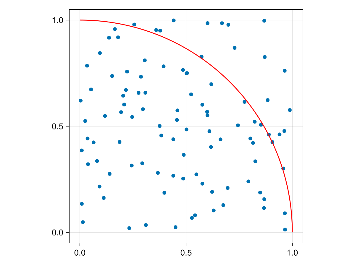
The fraction of points should be about the fraction of the area within the arc or \(\pi/4\text{.}\) (Note: the plot! function plots on top of the current plot instead of making a new one. It also performs a parametric plot--see Chapter 15--of the circle.)
Instead of just repeating the same code with a different number of points, we will create a function that estimates \(\pi\) based on the number of points originally.
function calcPi(total_points::Integer)
  pts=rand(total_points,2)
  dist=mapslices(pt -> pt[1]^2+pt[2]^2, pts; dims=[2])
  4*count(d -> d < 1,dist)/total_points
end
and we haven’t included the square root in the distance calculation because all we are trying to determine is which points are within the unit circle. This uses the square distance, so the result is the same.
Recall that earlier in the book, we determine that creating an array is one of the slower parts of code. In this case, it is not needed. Rewrite the calcPi function to not generate a matrix of total_points rows.
Write a for loop and inside the loop generate a single point and determine whether or not it is in the circle. Time this version and compare to the calcPi above.